Monday, 27 February 2017

MCA 4th sem /MCSP-044/Solved Assignment/Mini Project/2016-2017 New

Q.1.(a)Which System Development Life Cycle (SDLC) will you propose for the specification given above?

A.1.(a) SDLC is a process followed for a software project, within a software organization. It consists of a detailed plan describing how to develop, maintain, replace and alter or enhance specific software. The life cycle defines a methodology for improving the quality of software and the overall development process.
The following figure is a graphical representation of the various stages of a typical SDLC.


Stage 1: Planning and Requirement Analysis

Requirement analysis is the most important and fundamental stage in SDLC. It is performed by the senior members of the team with inputs from the customer, the medicine department, market surveys and domain experts in the industry. This information is then used to plan the basic project approach and to conduct product feasibility study in the economical, operational, and technical areas.

Stage 2: Defining Requirements

Once the requirement analysis is done the next step is to clearly define and document the product requirements and get them approved from the customer or the market analysts. This is done through .SRS. . Software Requirement Specification document which consists of all the product requirements to be designed and developed during the project life cycle.

Stage 3: Designing the product architecture

SRS is the reference for product architects to come out with the best architecture for the product to be developed. Based on the requirements specified in SRS, usually more than one design approach for the product architecture is proposed and documented in a DDS - Design Document Specification.

Stage 4: Building or Developing the Product

In this stage of SDLC the actual development starts and the product is built. The programming code is generated as per DDS during this stage. If the design is performed in a detailed and organized manner, code generation can be accomplished without much hassle.

Stage 5: Testing the Product

This stage is usually a subset of all the stages as in the modern SDLC models, the testing activities are mostly involved in all the stages of SDLC. However this stage refers to the testing only stage of the product where products defects are reported, tracked, fixed and retested, until the product reaches the quality standards defined in the SRS.

Stage 6: Deployment in the Market and Maintenance


Once the product is tested and ready to be deployed it is released formally in the appropriate market. Sometime product deployment happens in stages as per the organizations. business strategy. The product may first be released in a limited segment and tested in the real business environment (UAT- User acceptance testing).


Q.1.(b)Justify you selection by evaluating suitability of at least two SDLCs.


A.1.(b)
We select Spiral and V model for Medicine Store.

Causing for selecting spiral model:-
The spiral model combines the idea of iterative development with the systematic, controlled aspects of the waterfall model.
Spiral model is a combination of iterative development process model and sequential linear development model i.e. waterfall model with very high emphasis on risk analysis.
It allows for incremental releases of the product, or incremental refinement through each iteration around the spiral.


Causing for selecting V model:-
Under V-Model, the corresponding testing phase of the development phase is planned in parallel. So there are Verification phases on one side of the .V. and Validation phases on the other side. Coding phase joins the two sides of the V-Model.

Q.2.(a) What would be major costs of the system?

A.2.(a)  Costs
The newly implemented Medical store system created additional costs that were not incurred with the paper-chart system. There are 2 cost categories: the system costs and the induced costs. The system costs include the direct costs to build the system infrastructure, to develop the Medical Stores applications, and to purchase office supplies. The induced costs were required to smooth the Medical Store adoption. The first cost was to scan the existing paper-charts into the Medical Stores system. The second cost was to provide assistance to doctors through medical transcriptionists (MTs). MTs are typists who enter medical records into the Medical Stores system instead of the physicians at the point of care.

Q.2.(b)What may be the financial benefits of installing such a system?

A.2.(b)

1) More efficient operations
Because Medical Store management software provides an overview of day-to-day details such as patient appointments and staff reports, it serves as a helpful point of reference for tasks that have yet to be completed. Such systems also safeguard against forgetting important details, and can keep a checklist of yet-to-be-completed tasks. Because small Medical Stores often lack the resources of hospitals or larger offices, software can significantly help staff members manage their daily workflows.
2) Easier access to records
Medical Store management software stores important data in a safe, easily accessible location. Rather than using an outdated method such as a filing cabinet, such systems allow Medical Stores to keep digital copies of important information. If a doctor has a question about a referring physician, or a past medication, he or she can access the information almost instantly. Staff members can also easily find insurance and billing information. When team members can find relevant documents, the Medical Store can operate in an accurate, timely manner.
Many software systems are linked to electronic medical records. These records, of course, are used primarily for proper diagnosis and treatment. Having a digitalized copy of patient records allows providers to quickly access pertinent information in order to guarantee an accurate diagnosis. Many solo Medical Stores use free, cloud-based software, such as Kareo or Medical Store Fusion, which allow workers to easily schedule appointments, complete insurance, store patient information, and more. While Medical Stores can choose between traditional client-server and cloud-based alternatives, many prefer the flexibility that the latter option provides. If users need to access data remotely or want to avoid the cost associated with in-house servers, cloud-based systems are now a viable (and possibly superior) alternative.
3) Simplified billing
Medical Store management software allows Medical Stores to easily bill patients and process claims. Popular solutions, such as Epic’s Resolute Professional Billing system, allow users to easily complete financial transactions. They also provide an overview of past transactions. Many online Medical Store management systems can be integrated with patient portals or comprehensive EHRs, and allow patients to access their bills through a secure online site. This helps decrease payment time and keeps patients notified of any problems.
Medical Store management software helps medical offices run more smoothly, stores data in a safe location, and allows Medical Stores to easily bill patients. Proper implementation of the system will enable Medical Stores to transition from old, outdated methods to new methods. The system will improve efficiency and accuracy and provide easier access to relevant data. As such, it is a worthwhile investment for small Medical Stores.
Q.2.(c)Perform a cost-benefit analysis for the proposed software and report its findings.

A.2.(c) Cost-Benefit Analysis

In this study a CBA based on cash flows of SMC was carried out. The detailed items of costs and benefits were determined based on differential costing, which is mainly used for decision making in managerial accounting, after comparison of workflows between the paper-chart system and the Medical Store system. This was a conservative CBA in that this study excluded any potential or qualitative benefits . The financial costs and benefits were obtained primarily through the SMC accounting records. The costs of Medical Store implementation were the actual measured value. However, the benefits were calculated by using the difference between actual measured values and expected values without the Medical Store system. Therefore, when data were not available, capital amounts were determined by the opinions of experts, such as medical record administrators, care floor nurses, and IT engineers. The measured amounts were converted to present values (PV) using SMC's expected interest rate. Then, the net present value (NPV), the benefit-cost ratio (BCR), and the discounted payback period (DPP) were calculated.
Q.2.(d)List the major tasks and milestones of the Project and make a project schedule. You must make both GANTT and PERT charts. Explain the two charts drawn by you.

A.2.(d) 

Gantt Chart :-

The Gantt chart was first developed and introduced by Charles Gantt in 1917. It deals with the sequence of tasks needed to complete the project. In this chart, each horizontal bar represents a task. The length of the bar shows the time required to complete the task. On an X-Y chart, the X-axis stands for the time in which the project will get completed. The Gantt chart is a very effective tool in assessing a project’s status. It basically emphasizes and shows how much time is required for completing a task.

 Pert Chart:- 
Program Evaluation and Review Technique charts were developed and introduced in 1950 by the U.S. Navy. They were developed to manage large projects which had complex tasks and a very high intertask dependency. The charts have an initiation node, and the initiation node later branches into many networks of tasks.


Q.3.(a)Study the system and create a software requirement specification. You must identify either processes or objects while analyzing. During the analysis give consideration to possible input and output of the processes.

A.3.(a) 

Specific Requirements


The specific requirements are –

Functionality


Introduction –

This subsection contains the requirements for the e-store. These requirements are organized by the features discussed in the vision document. Features from vision documents are then refined into use case diagrams and to sequence diagram to best capture the functional requirements of the system. All these functional requirements can be traced using tractability matrix.

Sell Configured to Ordered Products.

The system shall display all the products that can be configured.

The system shall allow user to select the product to configure.

The system shall display all the available components of the product to configure

The system shall enable user to add one or more component to the configuration.

The system shall notify the user about any conflict in the current configuration.

The system shall allow user to update the configuration to resolve conflict in the current configuration.

The system shall allow user to confirm the completion of current configuration


Provide comprehensive product details. 

The system shall display detailed information of the selected products.

The system shall provide browsing options to see product details.

Detailed product Categorizations

The system shall display detailed product categorization to the user.

Provide Search facility.


The system shall enable user to enter the search text on the screen.

The system shall enable user to select multiple options on the screen to search.

The system shall display all the matching products based on the search

The system shall display only 10 matching result on the current screen.

The system shall enable user to navigate between the search results.

The system shall notify the user when no matching product is found on the search.

Maintain customer profile.

The system shall allow user to create profile and set his credential.

The system shall authenticate user credentials to view the profile.

The system shall allow user to update the profile information.

Q.3.(b)After identifying the requirements, create Analysis Models. You may either use the classical approach and draw Entity relationship diagram and data flow diagrams (DFD’s) up to level 2-3; 

or 

you may take object oriented analysis approach and create class diagram, use case diagram, use cases etc.

A.3.(b) We can create "Entity relationship diagram and data flow diagrams" , that are following :-

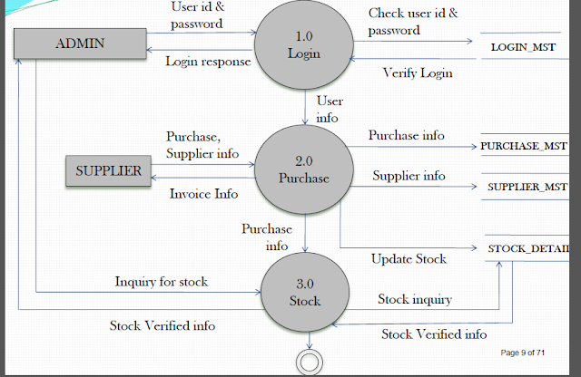
Context Level DFD:-


First Level DFD:-


Second Level DFD:-

Entity Relationship Diagram(ERD):-


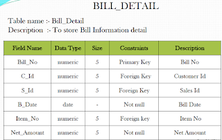
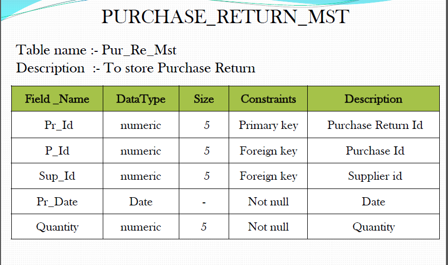
Q.4.(a) Design the system architecture and the database as per the needs of the system. You must perform normalization on relations up to 3rd normal form. The table design must include Primary and Foreign keys and constrains.

A.4.(a) Primary Key:-The PRIMARY KEY constraint uniquely identifies each record in a database table.
Primary keys must contain UNIQUE values.
A primary key column cannot contain NULL values.
Most tables should have a primary key, and each table can have only ONE primary key.

Foreign Key:-
A FOREIGN KEY in one table points to a PRIMARY KEY in another table.

Normal Forms :-
Database normalization is the process of efficiently organizing data in a database. There are two reasons of the normalization process:
  • Eliminating redundant data, for example, storing the same data in more than one tables.
  • Ensuring data dependencies make sense.
Both of these are worthy goals as they reduce the amount of space a database consumes and ensure that data is logically stored. Normalization consists of a series of guidelines that help guide you in creating a good database structure.
Normalization guidelines are divided into normal forms; think of form as the format or the way a database structure is laid out. The aim of normal forms is to organize the database structure so that it complies with the rules of first normal form, then second normal form, and finally third normal form.
It's your choice to take it further and go to fourth normal form, fifth normal form, and so on, but generally speaking, third normal form is enough.




Q.4.(b)Create the system flow chart or detailed process design and state transition diagrams. Also design the user input screens and output report formats.


A.4.(b) System Flow Chart  :-
System flowcharts are a way of displaying how data flows in a system and how decisions are made to control events.

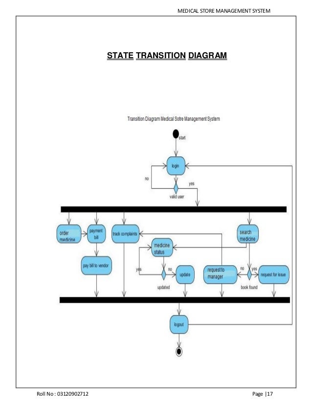
State Transition Diagram:-
State transition diagrams have been used right from the beginning in object-oriented modeling. The basic idea is to define a machine that has a number of states (hence the term finite state machine). The machine receives events from the outside world, and each event can cause the machine to transition from one state to another. For an example, take a look at figure 1. Here the machine is a bottle in a bottling plant. It begins in the empty state. In that state it can receive squirt events. If the squirt event causes the bottle to become full, then it transitions to the full state, otherwise it stays in the empty state (indicated by the transition back to its own state). When in the full state the cap event will cause it to transition to the sealed state. The diagram indicates that a full bottle does not receive squirt events, and that an empty bottle does not receive cap events. Thus you can get a good sense of what events should occur, and what effect they can have on the object.

Image result for state transition diagram for medical store management system

 INPUT DESIGN


OUTPUT DESIGN


Q.5.Design various unit test cases for different testing techniques/strategies.

A.5. 

Test case Design Technique

Following are the typical design techniques in software engineering:
1. Deriving test cases directly from a requirement specification or black box test design technique. The Techniques include:
·        Boundary Value Analysis (BVA)
·        Equivalence Partitioning (EP)
·        Decision Table Testing
·        State Transition Diagrams
·        Use Case Testing
2. Deriving test cases directly from the structure of a component or system:
·        Statement Coverage
·        Branch Coverage
·        Path Coverage
·        LCSAJ Testing
3. Deriving test cases based on tester's experience on similar systems or testers intuition:
·        Error Guessing
·        Exploratory Testing


Sunday, 26 February 2017

MCA4th Sem /MCS-042/Solved Assignment/Data Communication and Computer Network/2016-2017 New

Q.1.

A.1.
Dijkstra’s Algorithm

Dijkstra’s algorithm solves the single source shortest path problem on a weighted, directed graph only when all edge-weights are non-negative. It maintains a set S of vertices whose final shortest path from the source has already been determined and it repeatedly selects the left vertices with the minimum shortest-path estimate, inserts them into S, and relaxes all edges leaving that edge. In this we maintain a priority-Queue which is implemented via heap.

Steps  of Dijkstra's Algorithm for finding Shortest Path:-

Step 1) First we , choose Initial Point or Starting point of the path ,i.e. A.

We have many ways to reach from path A to  Target path  F , thar are the following:-

i)   A  ----> C --->  D----> F
ii)  A ---> B ---> E ---> F
iii)  A ---> E ---> F
iv)  A --->B 
But, we choose a shortest path to reach our Target path F. i.e
(i)  A  ----> C --->  D----> F 

Step 2) Starting from A , we choose Shortest path to F  , i.e.  A  ----> C


Step 3) Now , after (Starting from A , we choose Shortest path to F  , i.e.  A  ----> C)  we select path from  C --->  D


Step 4)  Now after Step 2 , we choose Shortest path to F  , i.e.  D  ----> F.


Step 4) Finish , we got our Target path in Shortest path. 


Q.2. Explain how a network congestion is controlled using slow start algorithm in TCP with help of an illustration. Is congestion control and flow control are equivalent?

A.2. Congestion control deals with adapting the source send rate to the bandwidth available to the transport connection, which varies over time in a non-predictable way because the network is shared by many applications. Consider the data flow from a TCP source to a TCP sink. The goal of TCP congestion control is three-fold:
  • To reduce the source send rate when the network is congested [more precisely, when the links on the network path of the TCP connection have queues that are growing very large].
  • To increase the source send rate when the network is not congested [so as to exploit bandwidth when it becomes available].
  • To share the network resources (i.e., link bandwidth and buffer) with other TCP flows in a "fair" way. There are many ways to quantify fairness. For example, consider a link of bandwidth C shared by n TCP flows. For i=1,...,n, let flow i want data rate B_i(t) at time t. Fairness is achieved if, at any time t, flow i gets data rate (B_i/B)*C if B_1(t)+...+B_n(t) exceeds C and data rate B_i otherwise. In practice, one can only approximate this.
Because TCP was designed to operate over unreliable heterogenous networks, its approach to congestion control relies on minimal knowledge of the network state. In particular, a TCP entity's knowledge about the current network state is derived solely from its recent history of message sends and receptions. Initial versions of TCP (e.g., Tahoe) used roundtrip times, where a roundtrip time is the time elapsed from sending a primary message (e.g., data message) to receiving an ack for that message. Later versions of TCP make use of the presence of duplicate acks (Reno) and the variation in the time intervals between acks (Vegas). In any case, TCP's view of the current network state is, to put it kindly, not very accurate. Consequently, TCP's congestion control must be very conservative.
The smoothest way to control the send rate is to directly adjust the time between successive packet sends. But TCP (like most computer software) does not operate at such "fine" time scales. Instead, TCP sends bursts of packets and adjusts its send rate by varying the number of packets in a burst. In a similar vein, TCP does not usually maintain separate timers for every outstanding packet (which would be needed to measure the roundtrip times of all primary packets [recall that a primary packet is one that is resent until a response is received]). Instead, TCP usually uses one timer to keep track of the last primary packet sent. If a primary packet is sent when the timer is running, it usually restarts the timer.

A TCP source entity does the following:
  • Maintains a running conservative estimate, called rto, of the current roundtrip time (by averaging recent roundtrip times and augmenting with some ``slack'').
  • Maintains a running estimate, called congestion window size, of how many packets can be sent without overloading the network path; the congestion window size never exceeds (and is usually much smaller) than the send window size.
  • Whenever a packet is acknowledged within rto, the entity increases the congestion window size and sends any new data that enters the congestion window. The increase is exponential if the congestion window is "small" (less than a so-called slow-start threshold), and linear otherwise.
  • Whenever a packet is not acknowledged within rto, the entity (treats this as an indication of congestion) decreases the congestion window to the minimum (thereby entering slow-start) and resends all data in the congestion window.
  • Whenever a packet loss is detected within rto, the entity decreases the congestion window by a multiplicative factor and resends the lost data.
Slow Start algorithm

Introduction
Jacobson and Karels developed a congestion control mechanism for TCP following a congestion collapse on the internet. Prior to this no congestion control mechanism was specified for TCP. Their method is based on ensuring the 'conservation of packets,' i.e., that the packets are entering the network at the same rate that they are exiting with a full window of packets in transit. A connection in this state is said to be in equilibrium. If all connections are in equilibrium, congestion collapse is unlikely The authors identified three ways for packet conservation to be violated:
1.     The connection never reaches equilibrium.
2.     A source sends a new packet before an old one exits.
3.     Congestion in the network prevents a connection from reaching equilibrium.
TCP is 'self clocking,' i.e., the source sends a new packet only when it receives an ack for an old one and the rate at which the source receives acks is the same rate at which the destination receives packets. So the rate at which the source sends matches the rate of transmission over the slowest part of the connection.

Algorithm
To ensure that the connection reaches equilibrium, i.e., to avoid failure (1), a slow-startalgorithm was developed. This algorithm added a congestion window. The minimum of the congestion windowand the destination window is used when sending packets. Upon starting a connection, or restarting after a packet loss, the congestion window size is set to one packet. The congestion window is then increased by one packet upon the receipt of an ack. This would bring the size of the congestion window to that of the destination window in RTT log W time, where RTT is the round-trip-time and W is the destination window size in packets. Without the slow start mechanism an 8 packet burst from a 10 Mbps LAN through a 56 Kbps link could put the connection into a persistent failure mode.
Violation (2) would occur if the retransmit time is too short, making the source retransmit a packet that has not been received and is not lost. What is needed is a good way to estimate the round trip time:
Err = Latest_RTT_Sample - RTT_Estimate
RTT_Estimate = RTT_Estimate + g*Err
where g is a 'gain' (0 < g < 1) which is related to the variance. This can be done quickly with integer arithmetic. This is an improvement over the previous method which used a constant to account for variance.
The authors also added exponential backoff for retransmitting packets that needed to be retransmitted more than once. This provides exponential dampening in the case where the round trip time increases faster than the RTT estimator can accommodate, and packets, which are not lost, are retransmitted.
Congestion avoidance takes care of violation (3). Lost packets are a good indication of congestion on the network. The authors state that the probability of a packet being lost due to transit is very rare. Furthermore, because of the improved round trip timer, it is a safe assumption that a timeout is due to network congestion. A additive increase / multiplicative decrease policy was used to avoid congestion.
Upon notification of network congestion, i.e., a timeout, the congestion window is set to half the current window size. Then for each ack for a new packet results in increasing the window by1/congestion_window_size. Note that if a packet times out, it is most likely that the source window is empty and nothing is being transmitted and a slow-start is required. In that case, the slow-start algorithm will increase the window (by one packet per ack) to half the previous window size, at which point the congestion avoidance algorithm takes over.

Performance

To test the effectiveness of their congestion control scheme, they compared their implementation of TCP to the previous implementation. They had four TCP conversations going between eight computers on two 10 Mbps LANs with a 230.4 Kbps link over the internet. They saw a 200% increase in effective bandwidth with the slow-start algorithm alone. The original implementation used only 35% of the available bandwidth due to retransmits. In another experiment, using the same network setup, the TCP implementation without congestion avoidance resulted in 4,000 of 11,000 packets sent were retransmitted packets as opposed to 89 of 8,281 with the new implementation.


Q.3.Describe how MACAW is an improvement over MACA ?

A.3.  A “media access protocol” is a link-layer protocol for allocating access to a shared medium (i.e. a wireless channel) among multiple transmitters. MACAW is a media access protocol for mobile pads that communicate wirelessly with base stations; each base station can hear transmission from pads within a certain range of its location, called a cell.
This is a challenging problem for several reasons:
§  Transmitters are mobile, but location information is not communicated explicitly: a transmitter simply moves or a new transmitter comes into the area, and the media access protocol must adapt.

§  Connectivity is not transitive. For example, A and B can communicate, as can B and C, but A and C might not be able to; the protocol must be designed so that communications between B and C do not disrupt A, even though A has no direct knowledge of C.

§  Due to noise, communication may not be symmetric (A can hear B, but B cannot hear A), and transmitters may interfere with one another (A might be out of range of B, but A’s transmissions might still disrupt B’s ability to communicate).

The MACAW paper ignores both asymmetry and interference: they assume a simplified model in which two stations are either in range of one another or they aren’t; a transmission is successfully received iff there is only one active transmitter in range of the receiver; and no two base stations are within range of one another. Importantly, contention between transmissions occurs at the receiver of the transmission, not the sender: that is, two nodes can transmit different messages from the same area at once, but two nodes in the same area cannot simultaneously receive different messages. Their goal is a media access protocol that is both efficient (high utilization of the available media), and fair (each station gets its “fair share”).
MACA:-

MACAW is an improved version of an earlier wireless media access protocol called MACA. MACA proceeds as follows:
§  Before sending a message, the transmitter sends a RTS control message (“ready to send”), containing the length of the upcoming data message. The time taken to transmit a control message (~30 bytes) is called a slot.
§  If the receiver hears the RTS and is not currently “deferring,” it replies with a CTS control message (“clear to send”), which includes a copy of the length field from the RTS.
§  Any station that hears a CTS defers any transmissions for long enough to allow someone to send a data message of the specified length. This avoids colliding with the CTS sender (the receiver of the upcoming data message).
§  Any station that hears an RTS defers any transmissions for a single slot (long enough for the reply CTS to be received, but not long enough for the actual data message to be sent, because contention is receiver-local).
§  Backoff: if no CTS response is received for an RTS, the sender must retransmit the RTS. It waits an integer number of slots before retransmitting, where that integer is chosen randomly between 1 and BO, the backoff counter. BO is doubled for every retransmit, and reduced to 1 for every successful RTS-CTS pair.

IMPROVEMENT
MACAW is proposed as a series of improvements to the basic MACA algorithm. First, they suggest a less aggressive backoff algorithm: the exponential increase / reset to 1 policy of MACA leads to large oscillations in the retransmission interval. They propose increasing BO by 1.5 after a timeout, and decreasing it by 1 after a successful RTS-CTS pair.
Second, they propose that receivers should send an ACK to the sender after successfully receiving a data message. This is suggested because the minimum TCP retransmission timeout is relatively long (0.5 seconds at the time), so it takes a long time to recover from lost or corrupted messages. A link layer timeout can be more aggressive, because it can take advantage of knowledge of the latency of the individual link (rather than the end-to-end timeout in TCP).

Q.4.Explain and illustrate sliding window Protocol with window size of 5. How does the scheme improve the efficiency of transmission ?

A.4. 
• In sliding window method, multiple frames are sent by sender at a time before needing an acknowledgment.

• Multiple frames sent by source are acknowledged by receiver using a single ACK frame.
Sliding Window


• Sliding window refers to an imaginary boxes that hold the frames on both sender and receiver side.


• It provides the upper limit on the number of frames that can be transmitted before requiring an acknowledgment.


• Frames may be acknowledged by receiver at any point even when window is not full on receiver side.


• Frames may be transmitted by source even when window is not yet full on sender side.


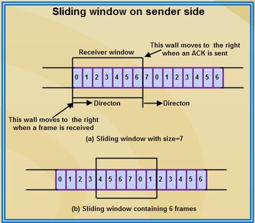
• The windows have a specific size in which the frames are numbered modulo- n, which means they are numbered from 0 to n-l. For e.g. if n = 8, the frames are numbered 0, 1,2,3,4,5,6, 7, 0, 1,2,3,4,5,6, 7, 0, 1, ....


• The size of window is n-1. For e.g. In this case it is 7. Therefore, a maximum of n-l frames may be sent before an acknowledgment.


• When the receiver sends an ACK, it includes the number of next frame it expects to receive. For example in order to acknowledge the group of frames ending in frame 4, the receiver sends an ACK containing the number 5. When sender sees an ACK with number 5, it comes to know that all the frames up to number 4 have been received. 


Sliding Window on Sender Side


• At the beginning of a transmission, the sender's window contains n-l frames.
• As the frames are sent by source, the left boundary of the window moves inward, shrinking the size of window. This means if window size is w, if four frames are sent by source after the last acknowledgment, then the number of frames left in window is w-4.
• When the receiver sends an ACK, the source's window expand i.e. (right boundary moves outward) to allow in a number of new frames equal to the number of frames acknowledged by that ACK.
• For example, Let the window size is 7 (see diagram (a)), if frames 0 through 3 have been sent and no acknowledgment has been received, then the sender's window contains three frames - 4,5,6.
• Now, if an ACK numbered 3 is received by source, it means three frames (0, 1, 2) have been received by receiver and are undamaged.
• The sender's window will now expand to include the next three frames in its buffer. At this point the sender's window will contain six frames (4, 5, 6, 7, 0, 1).

Sliding Window on Receiver Side 
• At the beginning of transmission, the receiver's window contains n-1 spaces for frame but not the frames.
• As the new frames come in, the size of window shrinks.
• Therefore the receiver window represents not the number of frames received but the number of frames that may still be received without an acknowledgment ACK must be sent.
• Given a window of size w, if three frames are received without an ACK being returned, the number of spaces in a window is w-3.
• As soon as acknowledgment is sent, window expands to include the number of frames equal to the number of frames acknowledged.
• For example, let the size of receiver's window is 7 as shown in diagram. It means window contains spaces for 7 frames.
• With the arrival of the first frame, the receiving window shrinks, moving the boundary from space 0 to 1. Now, window has shrunk by one, so the receiver may accept six more frame before it is required to send an ACK.
• If frames 0 through 3 have arrived but have DOC been acknowledged, the window will contain three frame spaces.
• As receiver sends an ACK, the window of the receiver expands to include as many new placeholders as newly acknowledged frames.
• The window expands to include a number of new frame spaces equal to the number of the most recently acknowledged frame minus the number of previously acknowledged frame. For e.g., If window size is 7 and if prior ACK was for frame 2 & the current ACK is for frame 5 the window expands by three (5-2).


Q.5.Explain the function and working model of Kerberos with the help of a diagram.

A.5. 

Kerberos is an authentication system based on private-key cryptography. In the Kerberos system, a trusted third-party issues session keys for interactions between users and services. It is mature technology which has been widely used, although it has known limitations. 

The Kerberos design is open-source, originating at MIT in the mid-1980's, and Kerberos is still freely available from MIT and other sources. Kerberos is also available in commercial software supported by vendors and has been incorporated into many widely-used products. For instance, Sun includes basic Kerberos functionality in Solaris, Cisco routers support Kerberos authentication for telnet connections, and Microsoft has announced it will use a version of the Kerberos protocol in Windows 2000. 

This paper will first list the goals and scope of the Kerberos system, followed by a brief review of concepts in private-key cryptography, and a description of the Kerberos "ticket-granting" approach. Appropriate applications, limitations, and competing technologies will be discussed, as well as the future of this technology. This brief overview of Kerberos is intended to highlight its main functionality, and does not exhaustively describe its features. For additional details on Kerberos, see the references listed at the end of this paper. 

Goals and Scope of the Kerberos system

Kerberos is designed to provide authentication of user identity in a networked computing environment consisting of workstations (used directly by one or more users) and servers (providing services such as email and shared file systems). It is, in part, a response to the current standard approach to network security, authentication by assertion, wherein a client gains access to services simply by asserting that it is who it says it is (or is acting on behalf of the user that it claims it is). 
A basic assumption is that network traffic is highly susceptible to interception and is the weak link in system security, rather than direct access to servers, which can be protected by physical means. The more often a specific cryptographic key is reused, the more susceptible it becomes to decoding. For this reason, each session of interactions between a user and a specific service should be encrypted using a short-lived "session key". To make the system usable in practice, however, it must be convenient, and to the greatest extent possible, transparent to the user. 
Starting with those assumptions, the system's key goals can be summarized as follows: 
  • Never transmit unencrypted passwords over the network, i.e. "in the clear". 
  • Protect against the misuse of intercepted credentials (also called "replay attacks"). 
  • Do not require the user to repeatedly enter a password to access routine services.
The Kerberos system attempts to address design tradeoffs between the level of protection provided and the user's convenience, while also considering the complexity of system administration and application development. 
Implementations of Kerberos are available from various vendors, and it is freely accessible in open-source form. The standard MIT distribution includes a basic set of applications, including telnet, POP email, and the Berkeley UNIX "R-commands" (such as rlogin). Other applications can be "Kerberized" by incorporating calls to Kerberos library functions. 

Encryption algorithms such as those used in Kerberos have long been considered munitions by the US government. The export status of Kerberos under newly liberalized regulations (October 2000) is unclear. For the time being, MIT is distributing its source only to US and Canadian citizens. Versions without encryption have been exported overseas, however. 


Q.6. Explain the process of generating a digital signature. What are its benefits ?

A.6. Digital signatures are the public-key primitives of message authentication. In the physical world, it is common to use handwritten signatures on handwritten or typed messages. They are used to bind signatory to the message.
Similarly, a digital signature is a technique that binds a person/entity to the digital data. This binding can be independently verified by receiver as well as any third party.
Digital signature is a cryptographic value that is calculated from the data and a secret key known only by the signer.
In real world, the receiver of message needs assurance that the message belongs to the sender and he should not be able to repudiate the origination of that message. This requirement is very crucial in business applications, since likelihood of a dispute over exchanged data is very high.

Model of Digital Signature

As mentioned earlier, the digital signature scheme is based on public key cryptography. The model of digital signature scheme is depicted in the following illustration −

The following points explain the entire process in detail −
·        Each person adopting this scheme has a public-private key pair.
·        Generally, the key pairs used for encryption/decryption and signing/verifying are different. The private key used for signing is referred to as the signature key and the public key as the verification key.
·        Signer feeds data to the hash function and generates hash of data.
·        Hash value and signature key are then fed to the signature algorithm which produces the digital signature on given hash. Signature is appended to the data and then both are sent to the verifier.
·        Verifier feeds the digital signature and the verification key into the verification algorithm. The verification algorithm gives some value as output.
·        Verifier also runs same hash function on received data to generate hash value.
·        For verification, this hash value and output of verification algorithm are compared. Based on the comparison result, verifier decides whether the digital signature is valid.
·        Since digital signature is created by ‘private’ key of signer and no one else can have this key; the signer cannot repudiate signing the data in future.


Importance of Digital Signature

Out of all cryptographic primitives, the digital signature using public key cryptography is considered as very important and useful tool to achieve information security.
Apart from ability to provide non-repudiation of message, the digital signature also provides message authentication and data integrity. Let us briefly see how this is achieved by the digital signature −
·        Message authentication − When the verifier validates the digital signature using public key of a sender, he is assured that signature has been created only by sender who possess the corresponding secret private key and no one else.
·        Data Integrity − In case an attacker has access to the data and modifies it, the digital signature verification at receiver end fails. The hash of modified data and the output provided by the verification algorithm will not match. Hence, receiver can safely deny the message assuming that data integrity has been breached.
·        Non-repudiation − Since it is assumed that only the signer has the knowledge of the signature key, he can only create unique signature on a given data. Thus the receiver can present data and the digital signature to a third party as evidence if any dispute arises in the future.


Q.7. What is called Constellation diagram ? Illustrate Constellation diagram of QAM – 16 and QAM – 64.

A.7. QAM, Quadrature amplitude modulation is widely used in many digital data radio communications and data communications applications. A variety of forms of QAM are available and some of the more common forms include 16 QAM, 32 QAM, 64 QAM, 128 QAM, and 256 QAM. Here the figures refer to the number of points on the constellation, i.e. the number of distinct states that can exist.
The various flavours of QAM may be used when data-rates beyond those offered by 8-PSK are required by a radio communications system. This is because QAM achieves a greater distance between adjacent points in the I-Q plane by distributing the points more evenly. And in this way the points on the constellation are more distinct and data errors are reduced. While it is possible to transmit more bits per symbol, if the energy of the constellation is to remain the same, the points on the constellation must be closer together and the transmission becomes more susceptible to noise. This results in a higher bit error rate than for the lower order QAM variants. In this way there is a balance between obtaining the higher data rates and maintaining an acceptable bit error rate for any radio communications system.

QAM applications

QAM is in many radio communications and data delivery applications. However some specific variants of QAM are used in some specific applications and standards.
For domestic broadcast applications for example, 64 QAM and 256 QAM are often used in digital cable television and cable modem applications. In the UK, 16 QAM and 64 QAM are currently used for digital terrestrial television using DVB - Digital Video Broadcasting. In the US, 64 QAM and 256 QAM are the mandated modulation schemes for digital cable as standardised by the SCTE in the standard ANSI/SCTE 07 2000.
In addition to this, variants of QAM are also used for many wireless and cellular technology applications.

Constellation diagrams for QAM

The constellation diagrams show the different positions for the states within different forms of QAM, quadrature amplitude modulation. As the order of the modulation increases, so does the number of points on the QAM constellation diagram.
The diagrams below show constellation diagrams for a variety of formats of modulation:
A diagram of the modulation constellation for BPSK showing the different positions adopted by the modulation points
a diagram of the modulation constellation for 16QAM showing the 16 modulation points


a diagram of the modulation constellation for 64QAM showing the 64 modulation points


Q.8.Differentiate between Leaky bucket and Token bucket traffic shaper. Why is traffic shaping needed ?
A.8 .Leaky Bucket 

 • Leaky bucket: consists of a finite queue – When a packet arrives, if there is a room on the queue it is joined the queue; otherwise, it is discarded – At every (fixed) clock tick, one packet is transmitted unless the queue is empty •
 It eliminates bursts completely: packets passed to the subnet at the same rate • 

This may be a bit overdone, and also packets can get lost (when bucket is full) Faucet Leaky bucket 
Water drips out of the hole at a constant rate Host computer Packet The bucket holds packets 
Unregulated flow Regulated flow Network Interface containing a leaky bucket Water .

Image result for leaky bucket image

• Token bucket: 

Tokens are added at a constant rate. For a packet to be transmitted, it must capture and destroy one token –

 (a) shows that the bucket holds three tokens with five packets waiting to be transmitted – (b) shows that three packets have gotten through but the other two are stuck waiting for tokens to be generated Host computer Networks Host computer The bucket holds tokens Networks One token is added to the bucket .
• Unlike leaky bucket, token bucket allows saving, up to maximum size of bucket n. This means that bursts of up to n packets can be sent at once, giving faster response to sudden bursts of input 
• An important difference between two algorithms: token bucket throws away tokens when the bucket is full but never discards packetswhile leaky bucket discards packets when the bucket is full .

• Let token bucket capacity be C (bits), token arrival rate ρ (bps), maximum output rate M (bps), and burst length S (s) – During burst length of S (s), tokens generated are ρS (bits), and output burst contains a maximum of C + ρS (bits) – Also output in a maximum burst of length S (s) is M · S (bits), thus C + ρS = MS or S = C M − ρ 
• Token bucket still allows large bursts, even though the maximum burst length S can be regulated by careful selection of ρ and M 
• One way to reduce the peak rate is to put a leaky bucket of a larger rate (to avoid discarding packets) after the token bucket.

Image result for token bucket image


Q.9.Assume we need to download a text document at a rate of 100 pages per minute. What is required bit rate of the channel. 
Assume Page size = 24 lines
 Each line = 81 characters

A.9. 
Relationship between Bandwidth, Data Rate and Channel Capacity
This posts describes the relationship between signal bandwidth, channel bandwidth and maximum achievable data rate. Before, going into detail, knowing the definitions of the following terms would help:

Signal Bandwidth – the bandwidth of the transmitted signal or the range of frequencies present in the signal, as constrained by the transmitter.

Channel Bandwidth – the range of signal bandwidths allowed by a communication channel without significant loss of energy (attenuation).

Channel Capacity or Maximum Data rate – the maximum rate (in bps) at which data can be transmitted over a given communication link, or channel.

In general, information is conveyed by change in values of the signal in time.  Since frequency of a signal is a direct measure of the rate of change in values of the signal, the more the frequency of a signal, more is the achievable data rate or information transfer rate. This can be illustrated by taking the example of both an analog and a digital signal.
If we take analog transmission line coding techniques like Binary ASK, Binary FSK or Binary PSK, information is tranferred by altering the property of a high frequency carrier wave. If we increase the frequency of this carrier wave to a higher value, then this reduces the bit interval T (= 1/f) duration, thereby enabling us to transfer more bits per second.

Similarly, if we take digital transmission techniques like NRZ, Manchester encoding etc., these signals can be modelled as periodic signals and hence is composed of an infinite number of sinusoids, consisting of a fundamental frequency (f) and its harmonics. Here too, the bit interval (T) is equal to the reciprocal of the fundamental frequency (T =  1/f). Hence, if the fundamental frequency is increased, then this would represent a digital signal with shorter bit interval and hence this would increase the data rate.

So, whether it is analog or digital transmission, an increase in the bandwidth of the signal, implies a corresponding increase in the data rate. For e.g. if we double the signal bandwidth,  then the data rate would also double.

In practise however, we cannot keep increasing the signal bandwidth infinitely. The telecommunication link or the communication channel acts as a police and has limitations on the maximum bandwidth that it would allow. Apart from this, there are standard transmission constraints in the form of different channel noise sources that strictly limit the signal bandwidth to be used.  So the achievable data rate is influenced more by the channel’s bandwidth and noise characteristics than the signal bandwidth.


Nyquist and Shannon have given methods for calculating the channel capacity (C) of bandwidth limited communication channels.

Solution 

A page is an average of 24 lines with 80 characters in each line. If we assume that one character requires 8 bits, the bit rate is:

   100 X 81 X 24 X 8 = 1555200 bps)Bit per second) = 1.555 Mbps

Q.10.Find CRC for the data polynomial x9 + x7 + x3 +x2 + 1 with generator polynomial x3 + x + 1.

A.10  


Cyclic Redundancy Check (CRC) An error detection mechanism in which a special number is appended to a block of data in order to detect any changes introduced during storage (or transmission). The CRe is recalculated on retrieval (or reception) and compared to the value originally transmitted, which can reveal certain types of error. For example, a single corrupted bit in the data results in a one-bit change in the calculated CRC, but multiple corrupt bits may cancel each other out.

A CRC is derived using a more complex algorithm than the simple CHECKSUM, involving MODULO ARITHMETIC (hence the 'cyclic' name) and treating each input word as a set of coefficients for a polynomial.

• CRC is more powerful than VRC and LRC in detecting errors.
• It is not based on binary addition like VRC and LRC. Rather it is based on binary division.
• At the sender side, the data unit to be transmitted IS divided by a predetermined divisor (binary number) in order to obtain the remainder. This remainder is called CRC.
• The CRC has one bit less than the divisor. It means that if CRC is of n bits, divisor is of n+ 1 bit.
• The sender appends this CRC to the end of data unit such that the resulting data unit becomes exactly divisible by predetermined divisor i.e. remainder becomes zero.
• At the destination, the incoming data unit i.e. data + CRC is divided by the same number (predetermined binary divisor).
• If the remainder after division is zero then there is no error in the data unit & receiver accepts it.
• If remainder after division is not zero, it indicates that the data unit has been damaged in transit and therefore it is rejected.
• This technique is more powerful than the parity check and checksum error detection.
• CRC is based on binary division. A sequence of redundant bits called CRC or CRC remainder is appended at the end of a data unit such as byte. 


Q.11.Suppose you are developing a standard for a new type of a network. You need to decide whether your network will use Virtual Circuits (VCs) or datagram routing. What are the Pros & Cons for using VCs ?

A.11.Datagrams and Virtual Circuits
Two basic approaches to packet switching are common: The most common is datagram switching (also known as a "best-effort network" or a network supporting the connection-less network service).This is what is used in the network layer of Internet.
Virtual circuit is a connection which is oriented unlike datagram switching. The source and destination identifies a suitable path for virtual circuit before the actual data communication starts. For this, it makes use of all intermediate nodes, routing table and other additional parameters. 

Once the data transmission is completed, the resources and values present for the virtual circuit are removed completely. There are two categories of virtual circuit, namely switched virtual circuit and permanent virtual circuit.

Switched virtual circuit is a virtual circuit in the connection is dynamically established based on the demand and is torn down completely once the transmission is complete. Permanent virtual circuit is one provided for continuous usage or repeated usage between the dame data terminals.

Virtual Circuit Packet Networks

In virtual circuit packet switching, an initial setup phase is used to set up a fixed route between the intermediate nodes for all packets which are exchanged during a session between the end nodes (analogous to the circuit-switched telephony network). At each intermediate node, an entry is made in a table to indicate the route for the connection that has been set up. Packets can then use short headers, since only identification of the virtual circuit rather than complete destination address is needed. The intermediate nodes (B,C) process each packet according to the information which was stored in the node when the connection was established.
Enhancements to provide reliability may also be provided. Delivery of packets in proper sequence and with essentially no errors is guaranteed, and congestion control to minimise queuing is common. Delays are more variable than they are with a dedicated circuit, however, since several virtual circuits may compete for the same resources. An initial connection setup phase and a disconnect phase at the end of data transfer are required (as in the circuit-switched network). The most common form of virtual circuit network were ATM and X.25, which for a while were commonly used for public packet data networks.
A variation of circuit-switched packet networking, called Multi-Protocol Label Switching (MPLS), is used in some Internet backbones. This uses a connection-oriented datagram service to switch packets across a network forming a path between a set of IP routers. This operates below the network-layer, so that applications are unaware of when MPLS is used.

Differences between datagram and virtual circuit networks

There are a number of important differences between virtual circuit and datagram networks. The choice strongly impacts complexity of the different types of node. Use of datagrams between intermediate nodes allows relatively simple protocols at this level, but at the expense of making the end (user) nodes more complex when end-to-end virtual circuit service is desired.
The Internet transmits datagrams between intermediate nodes using IP. Most Internet users need additional functions such as end-to-end error and sequence control to give a reliable service (equivalent to that provided by virtual circuits). This reliablility may be provided by the Transmission Control Protocol (TCP) which is used end-to-end across the Internet, or by applications such as the trivial file transfer protocol (tftp) running on top of the User Datagram Protocol (UDP).

Q.12.Why is that packet switching is said to employ statistical multiplexing ? Contrast statistical multiplexing with the multiplexing that take place in TDM.

A.12.
Statistical multiplexing is a type of communication link sharing, very similar to dynamic bandwidth allocation (DBA). In statistical multiplexing, a communication channel is divided into an arbitrary number of variable bitrate digital channels or data streams. The link sharing is adapted to the instantaneous traffic demands of the data streams that are transferred over each channel. This is an alternative to creating a fixed sharing of a link, such as in general time division multiplexing (TDM) and frequency division multiplexing (FDM). When performed correctly, statistical multiplexing can provide a link utilization improvement, called the statistical multiplexing gain.

Statistical multiplexing is facilitated through packet mode or packet-oriented communication, which among others is utilized in packet switched computer networks. Each stream is divided into packets that normally are delivered asynchronously in a first-come first-served fashion. In alternative fashion, the packets may be delivered according to some scheduling discipline for fair queuing or differentiated and/or guaranteed quality of service.

Statistical multiplexing of an analog channel, for example a wireless channel, is also facilitated through the following schemes:

Random frequency-hopping orthogonal frequency division multiple access (RFH-OFDMA)
Code-division multiple access (CDMA), where different amount of spreading codes or spreading factors can be assigned to different users.
Statistical multiplexing normally implies "on-demand" service rather than one that preallocates resources for each data stream. Statistical multiplexing schemes do not control user data transmissions.

Comparison with static TDM

Time domain statistical multiplexing (packet mode communication) is similar to time-division multiplexing (TDM), except that, rather than assigning a data stream to the same recurrent time slot in every TDM, each data stream is assigned time slots (of fixed length) or data frames (of variable lengths) that often appear to be scheduled in a randomized order, and experience varying delay (while the delay is fixed in TDM).

Statistical multiplexing allows the bandwidth to be divided arbitrarily among a variable number of channels (while the number of channels and the channel data rate are fixed in TDM).

Statistical multiplexing ensures that slots will not be wasted (whereas TDM can waste slots). The transmission capacity of the link will be shared by only those users who have packets.

Static TDM and other circuit switching is carried out at the physical layer in the OSI model and TCP/IP model, while statistical multiplexing is carried out at the data link layer and above.

Channel identification


In statistical multiplexing, each packet or frame contains a channel/data stream identification number, or (in the case of datagram communication) complete destination address information.