Ans 1:
Insertion Sort Algorithm
- ·
Get
a list of unsorted numbers
- ·
Set
a marker for the sorted section after the first number in the list
- ·
Repeat
steps 4 through 6 until the unsorted section is empty
- ·
Select
the first unsorted number
- ·
Swap
this number to the left until it arrives at the correct sorted position
- ·
Advance
the marker to the right one position
- ·
Stop
Best Complexity of
Insertion Sort is : O(n)
Average Complexity of
Insertion Sort is : O(log n)
Worst Complexity of
Insertion Sort is : O(n2)
/*
insertion sort ascending order */
#include <stdio.h>
int main()
{
int n, array[1000], c, d, t;
printf("Enter
number of elements\n");
scanf("%d", &n);
printf("Enter
%d integers\n", n);
for (c = 0; c < n; c++) {
scanf("%d", &array[c]);
}
for (c = 1 ; c <= n - 1; c++) {
d = c;
while ( d > 0 && array[d] < array[d-1]) {
t = array[d];
array[d]
= array[d-1];
array[d-1] = t;
d--;
}
}
printf("Sorted
list in ascending order:\n");
for (c = 0; c <= n - 1; c++) {
printf("%d\n", array[c]);
}
return 0;
}
ANS 2)
(i) Pseudo code
minIndex=1
min=A[1]
i=0
while(i <= n)
if A[i]<min
min=A[i]
minIndex = i
i+=1
#include<stdio.h>
int main()
{
int a[30], i, num, smallest;
printf("\nEnter no of elements :");
scanf("%d", &num);
//Read n elements in an array
for (i = 0; i < num; i++)
scanf("%d",
&a[i]);
//Consider first element as smallest
smallest = a[0];
for (i = 0; i < num; i++) {
if
(a[i] < smallest) {
smallest = a[i];
}
}
// Print out the Result
printf("\nSmallest Element : %d", smallest);
return (0);
}
|
OUTPUT:
1
2
3
|
Enter no of elements : 5
11 44 22 55 99
Smallest Element : 11
|
ii) Pseudo CODE
use the following method:
mark the missing number as M
and the duplicated as D
1) compute the sum of
regular list of numbers from 1 to N call it RegularSum
2) compute the sum of your
array (the one with M and D) call it MySum
now you know that
MySum-M+D=RegularSum
this is one equation.
the second one uses
multiplication:
3) compute the
multiplication of numbers of regular list of numbers from 1 to N call it
RegularMultiplication
4) compute the
multiplication of numbers of your list (the one with M and D) call it
MyMultiplication
now you know that
MyMultiplication=RegularMultiplication*D/M
at this point you have two
equations with two parameters, solve and rule!
int
findPos(int arr[], int key)
{
int
l = 0, h = 1;
int
val = arr[0];
//
Find h to do binary search
while
(val < key)
{
l
= h; // store previous high
h
= 2*h; // double high index
val
= arr[h]; // update new val
}
return
binarySearch(arr, l, h, key);
}
// Driver
program
int main()
{
int
arr[] = {3, 5, 7, 9, 10, 90, 100, 130,
140,
160, 170};
int
ans = findPos(arr, 10);
if
(ans==-1)
cout
<< "Element not found";
else
cout
<< "Element found at index " << ans;
return
0;
}
|
Run on IDE
Output:
Element found
at index 4
Ans 3)
QuickSort
Like Merge
Sort, QuickSort is a Divide and Conquer algorithm. It picks an element as pivot
and partitions the given array around the picked pivot. There are many
different versions of quickSort that pick pivot in different ways.
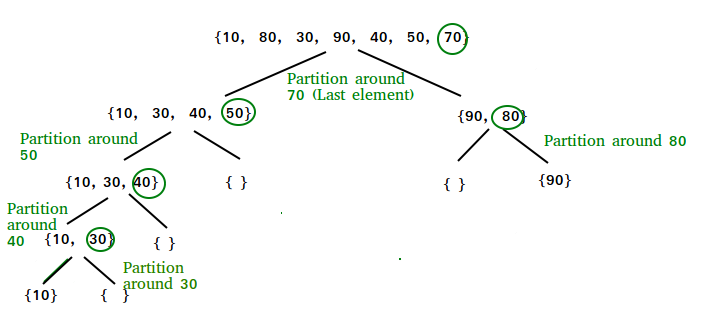
Always pick
first element as pivot.
Always pick
last element as pivot (implemented below)
Pick a random
element as pivot.
Pick median
as pivot.
The key
process in quickSort is partition(). Target of partitions is, given an array
and an element x of array as pivot, put x at its correct position in sorted
array and put all smaller elements (smaller than x) before x, and put all
greater elements (greater than x) after x. All this should be done in linear
time.
Pseudo Code
for recursive QuickSort function :
/* low --> Starting index, high
--> Ending index */
quickSort(arr[],
low, high)
{
if (low < high)
{
/* pi is partitioning index, arr[p] is
now
at right place */
pi = partition(arr, low, high);
quickSort(arr, low, pi - 1); // Before pi
quickSort(arr, pi + 1, high); // After
pi
}
}
Partition
Algorithm
There can be many ways to do partition, following pseudo code adopts the method
given in CLRS book. The logic is simple, we start from the leftmost element and
keep track of index of smaller (or equal to) elements as i. While traversing,
if we find a smaller element, we swap current element with arr[i]. Otherwise we
ignore current element.
/* low --> Starting index, high
--> Ending index */
quickSort(arr[],
low, high)
{
if (low < high)
{
/* pi is partitioning index, arr[p] is
now
at right place */
pi = partition(arr, low, high);
quickSort(arr, low, pi - 1); // Before pi
quickSort(arr, pi + 1, high); // After
pi
}
}
Pseudo code
for partition()
partition
(arr[], low, high)
{
// pivot (Element to be placed at right
position)
pivot = arr[high];
i = (low - 1) // Index of smaller element
for (j = low; j <= high- 1; j++)
{
// If current element is smaller than
or
// equal to pivot
if (arr[j] <= pivot)
{
i++; // increment index of smaller element
swap arr[i] and arr[j]
}
}
swap arr[i + 1] and arr[high])
return (i + 1)
}
Difference between Quick Sort Randrandomized Quich Sort
Randomized Quick Sort differs from Quick Sort in how it selects
pivots. This doesn’t eliminate the possibility of
worst-case behavior, but it removes the ability of any specific input to
reliably and consistently cause that worst-case behavior.
How does it do this?
‘RQS’ chooses a random pivot rather than
selecting the first, last, middle, median of those, median-of-medians, or some
other technique.
The cost of random number generation for pivot index selection
is negligible, plus two-reads-and-a-write for the actual pivot swap with
front-of-range. During Quick Sort, each element is chosen as a pivot either
once or not at all, leading to a low overall cost of O(n) for random pivot
selection. The only cheaper techniques are the “dumb & dumber” options of
always choosing last or first index.
So it’s cheap, but does it improve the worst-case performance?
Well, yes and no. There is still a theoretical possibility
of O(n^2) behavior, but not in any consistent way.
Randomized Quick Sort — what is it good for?
Randomized Quick Sort removes any determinism or repeatability
from worst-case behaviors. For every possible input, the
expected run-time is O(n logn), because selecting a pivot randomly is like
randomizing the array every time.
With RQS, there is a hypothetical chance of being colossally
unlucky and randomly selecting an anti-pivot at every turn, but the chance of
this happening are lower than the chance of your being struck by lightning, and
then winning the lottery.
This differs from Quick Sort where certain specific
inputs cause bad performance every single time — something a malicious
actor could exploit by sending anti-sorted data.
That’s
why Randomized Quick Sort is effectively much more
efficient in worst-case.
Worst Case Analysis
WORST CASE ANALYSIS:
Now consider the case, when the pivot happened
to be the least element of the array, so that we had k = 1 and n − k = n − 1.
In such a
case, we have:
T(n) = T(1) +
T(n − 1) + αn Now let us analyse the time complexity of quick sort in such a
case in detail by solving the recurrence as follows:
T(n) = T(n − 1) + T(1) + αn = [T(n − 2) + T(1)
+ α(n − 1)] + T(1) + αn
I have
written T(n − 1) = T(1) + T(n − 2) + α(n − 1) by just substituting n − 1
instead of n.
Note the implicit assumption that the pivot
that was chosen divided the original subarray of size n − 1 into two parts: one
of size n − 2 and the other of size 1.) =
T(n − 2) +
2T(1) + α(n − 1 + n) (by simplifying and grouping terms together)
= [T(n − 3) + T(1) + α(n − 2)] + 2T(1) + α(n −
1 + n)
= T(n − 3) +
3T(1) + α(n − 2 + n − 1 + n)
= [T(n − 4) +
T(1) + α(n − 3)] + 3T(1) + α(n − 2 + n − 1 + n)
Alphabetical Order:-
#include <ctype.h>
#include <string>
#include <iostream>
#include <cstring>
#include <iomanip>
#include <stdio.h>
using namespace std;
const int DATA = 1000;
int compare(const void* , const
void*);
int main()
{
int i;
int m;
int j;
int n;
char c;
char list[DATA];
string word[100];
cout << "Enter words:\n";
fgets (list, 256, stdin );
printf ("You entered: ");
cout << endl;
printf (list);
cout << endl;
while (list[i])
{
if (isupper(list[i])) list[i]=tolower(list[i]);
putchar (list[i]);
i++;
}
cout << endl;
qsort(list, DATA, sizeof(char),
compare);
cout << endl;
cout << "The sorted list of words:\n";
printf (list);
cout << endl;
return 0;
}
int compare(const void* pnum1, const void *pnum2)
// compares two numbers, returns -1
if first is smaller
// returns 0 is they are equal,
returns 1 if first is larger
{
int num1, num2;
num1 = *(char *)pnum1; // cast
from pointer to void
num2 = *(char *)pnum2; // to
pointer to int
if(num1 < num2)
return -1;
else
if (num1 == num2)
return 0;
else
return 1;
}
Ans 4)
Dynamic Programming has similarities with backtracking and
divide-conquer in many respects. Here is how we generally solve a problem using
dynamic programming.
- Split
the problem into overlapping sub-problems.
- Solve
each sub-problem recursively.
- Combine
the solutions to sub-problems into a solution for the given problem.
- Don’t
compute the answer to the same problem more than once.
Let us devise a program to calculate nth Fibonacci number.
Let us solve this recursively.
int fibo(int
n)
{
if(n<=2)
return 1;
else
return fibo(n-2)+fibo(n-1);
}
The complexity of the above program would be exponential
Now let are solve this problem dynamically.
int
memory[500]
memset(memory,
-1 ,500)
int fibo(int
n) {
if(n<=2)
return 1;
if(memory[n]!=-1)
return memory[n];
int
s=fibo(n-1)+fibo(n-2);
memory[n]=s;
return s;
}
We have n possible inputs to the function: 1, 2, …, n. Each
input will either:–
1.
be computed, and the result saved
2.
be returned from the memory
Each input will be computed at most once Time complexity is O(n
× k), where k is the time complexity of computing an input if we assume that the
recursive calls are returned directly from memory(O(1))
Since we’re only doing constant amount of work tocompute the
answer to an input, k = O(1)
Total time complexity is O(n).
Algorithm To Determine Optimal Parenthesization of a
Product of N Matrices
Input n matrices.
Separate it into two
sub-sequences.
Find out the minimum cost of
multiplying every set.
Calculate the sum of these
costs, and add in the cost of multiplying the two matrices.
Repeat the above steps for
every possible position at which the sequence of matrices can split, and take
the minimum cost.
Optimality Principle
The influence of Richard
Bellman is seen in algorithms throughout the computer science literature.
Bellman’s principle of optimality has been used to develop highly efficient dynamic
programming solutions to many important and difficult problems. The paradigm is
now well entrenched as one of the most successful algorithm design tools
employed by computer scientists.
The optimality principle was
given a broad and general statement by Bellman [23, making it applicable to
problems of diverse types. Since computer programs are often employed to
implement solutions based on the principle of optimality, Bellman’s impact on
computing in general has been immense. In this paper we wish to focus in
particular on the influence of Bellman’s work on the area of computer science
known as algorithm design and analysis. A primary goal of algorithm design and
analysis is to discover theoretical properties of classes of algorithms (e.g.,
how efficient they are, when they are applicable) and thus learn how to better
apply the algorithms to new problems. From the perspective of algorithm design
and analysis, combinatorial optimization problems form the class of problems on
which the principle of optimality has had its greatest impact. Problem
decomposition is a basic technique for attacking problems of this type-the
solution to a large problem is obtained by combining solutions to smaller
subproblems. The trick of this approach, of course, is to define an efficient
decomposition procedure which assures that combining optimal solutions to
subproblems will result in an optimal solution to the larger problem. As a
standard course of action, computer scientists attempt to define a
decomposition based on Bellman’s principle of optimality. Problem
decompositions based on the principle of optimality not only are at the heart
of dynamic programming algorithms, but are also integral parts of the
strategies of other important classes of algorithms, such as branch and bound.
Matrix Multiplication
A1*A2 => 30* 35
=> 1050
A2*A3 => 35*15
=> 525
A3*A1 => 15 *5
=> 75
A2 A3 A1
A1 (1050)
A2 (525)
A3 (75)
Ans 5 i)
Greedy technique and Dynamic programming technique
Greedy
|
Dynamic Programming
|
A
greedy algorithm is one that at a given point in time, makes a local optimization.
|
Dynamic programming can be thought of as
'smart' recursion.,It often requires one to break down a problem into smaller
components that can be cached.
|
Greedy algorithms have a local choice of the
subproblem that will lead to an optimal answer
|
Dynamic programming would solve all
dependent subproblems and then select one that would lead to an optimal
solution.
|
A
greedy algorithm is one which finds optimal solution at each and every stage
with the hope of finding global optimum at the end.
|
A Dynamic algorithm is applicable to
problems that exhibit Overlapping subproblems and Optimal substructure
properties.
|
More
efficient as compared,to dynamic programming
|
Less efficient as compared to greedy
approach
|
ii) NP-Complete & NP Hard Problems
NP-Complete:
NP-Complete is a complexity
class which represents the set of all problems X in NP for which it is possible
to reduce any other NP problem Y to X in polynomial time.
Intuitively this means that
we can solve Y quickly if we know how to solve X quickly. Precisely, Yis
reducible to X, if there is a polynomial time algorithm f to transform
instances y of Y to instances x = f(y) of X in polynomial time, with the
property that the answer to y is yes, if and only if the answer to f(y) is yes.
Example
3-SAT. This is the problem wherein we are given a
conjunction (ANDs) of 3-clause disjunctions (ORs), statements of the form
(x_v11 OR x_v21 OR x_v31) AND
(x_v12 OR x_v22 OR x_v32) AND
...
AND
(x_v1n OR x_v2n OR x_v3n)
where each x_vij is a boolean variable or the
negation of a variable from a finite predefined list (x_1, x_2, ... x_n).
It can be shown that every NP problem
can be reduced to 3-SAT. The proof of this is technical and requires use of
the technical definition of NP (based on non-deterministic Turing machines).
This is known as Cook's theorem.
What makes NP-complete problems important is
that if a deterministic polynomial time algorithm can be found to solve one of
them, every NP problem is solvable in polynomial time (one problem to rule them
all).
NP-hard
Intuitively, these are the problems that are at
least as hard as the NP-complete problems. Note that NP-hard problems do
not have to be in NP, and they do not have to be decision problems.
The precise definition here is
that a problem X is
NP-hard, if there is an NP-complete problem Y, such that Y is
reducible to X in
polynomial time.
But since any NP-complete problem can be reduced to
any other NP-complete problem in polynomial time, all NP-complete problems can
be reduced to any NP-hard problem in polynomial time. Then, if there is a
solution to one NP-hard problem in polynomial time, there is a solution to all
NP problems in polynomial time.
Example
The halting problem is
an NP-hard problem. This is the problem that given a program P and input I, will it halt? This is a decision problem but it is not in
NP. It is clear that any NP-complete problem can be reduced to this one. As
another example, any NP-complete problem is NP-hard.
iii) Decidable & Un-decidable problems
A language is
called Decidable or Recursive if there is a
Turing machine which accepts and halts on every input string w.
Every decidable language is Turing-Acceptable.
A decision
problem P is decidable if the language L of
all yes instances to P is decidable.
For a decidable
language, for each input string, the TM halts either at the accept or the
reject state.
Example
Solution
- The halting problem of Turing
machine
- The mortal matrix problem
- The Post correspondence
problem, etc.
Find out whether the following problem is decidable or not −
Is a number ‘m’ prime?
Prime numbers = {2, 3, 5, 7, 11, 13, …………..}
Divide the number ‘m’ by all the numbers between
‘2’ and ‘√m’ starting from ‘2’.
If any of these numbers produce a remainder zero, then it goes to
the “Rejected state”, otherwise it goes to the “Accepted state”. So, here the
answer could be made by ‘Yes’ or ‘No’.
Hence, it is a decidable problem.
or an undecidable
language, there is no Turing Machine which accepts the language and makes a
decision for every input string w (TM can make decision for
some input string though). A decision problem P is called
“undecidable” if the language L of all yes instances to P is
not decidable. Undecidable languages are not recursive languages, but
sometimes, they may be recursively enumerable languages.
iv)
Context free & Context sensitive Language
Context free language:
In formal
language theory, a context-free language (CFL) is a language generated
by a context-free grammar (CFG).
Definition − A
context-free grammar (CFG) consisting of a finite set of grammar rules is a
quadruple (N, T, P, S) where
·
N is a set of non-terminal symbols.
·
T is a set of terminals where N
∩ T = NULL.
·
P is a set of rules, P: N →
(N ∪ T)*, i.e., the left-hand side of the
production rule P does have any right context or left context.
·
S is the start symbol.
Example
- The grammar ({A}, {a, b, c},
P, A), P : A → aA, A → abc.
- The grammar ({S, a, b}, {a,
b}, P, S), P: S → aSa, S → bSb, S → ε
- The grammar ({S, F}, {0, 1},
P, S), P: S → 00S | 11F, F → 00F | ε
Context
sensitive Language
In theoretical computer science, a context-sensitive language is
a formal language that can be
defined by a context-sensitive grammar (and
equivalently by a noncontracting grammar). Context-sensitive is one of the four types of grammars in
the Chomsky hierarchy.
Type-1 grammars generate context-sensitive languages. The productions must
be in the form
α A β → α γ β
where A ∈ N (Non-terminal)
and α, β, γ ∈ (T ∪ N)* (Strings of terminals and non-terminals)
The strings α and β may be
empty, but γ must be non-empty.
The rule S → ε is allowed if S does not appear on
the right side of any rule. The languages generated by these grammars are
recognized by a linear bounded automaton.
Example
AB → AbBc
A → bcA
B → b
v) Strassen’s Algorithm & Chain
Matrix Multiplication algorithm
Strassen’s Algorithm
In linear
algebra, the Strassen algorithm, named
after Volker Strassen, is an algorithm
for matrix multiplication. It is faster than the
standard matrix multiplication algorithm and is useful in practice for large
matrices, but would be slower than the fastest known algorithms for extremely large matrices.
Strassen's algorithm works for any ring, such as plus/multiply, but not all semirings, such as min/plus or boolean
algebra, where the naive algorithm still works, and so called combinatorial matrix multiplication.
Complexity
As
I mentioned above the Strassen’s algorithm is slightly faster than the general
matrix multiplication algorithm. The general algorithm’s time complexity is
O(n^3), while the Strassen’s algorithm is O(n^2.80).
You
can see on the chart below how slightly faster is this even for large n.
Chain Matrix Multiplication
algorithm:
Matrix chain multiplication (or Matrix Chain Ordering Problem, MCOP) is an optimization
problem that can be solved using dynamic
programming. Given a sequence of matrices, the goal
is to find the most efficient way to multiply these matrices. The problem is not actually to perform the
multiplications, but merely to decide the sequence of the matrix
multiplications involved.
Following is C/C++ implementation for Matrix
Chain Multiplication problem using Dynamic Programming.
#include<stdio.h>
#include<limits.h>
// Matrix Ai has dimension p[i-1] x p[i] for i = 1..n
int MatrixChainOrder(int p[], int n)
{
/* For simplicity of the program, one extra row
and one
extra column are allocated in
m[][]. 0th row and 0th
column of m[][] are not used
*/
int m[n][n];
int i, j, k, L, q;
/* m[i,j] = Minimum number of scalar
multiplications needed
to compute the matrix
A[i]A[i+1]...A[j] = A[i..j] where
dimension of A[i] is p[i-1] x
p[i] */
// cost is zero when multiplying one matrix.
for (i=1; i<n; i++)
m[i][i] = 0;
// L is chain length.
for (L=2; L<n; L++)
{
for (i=1; i<n-L+1;
i++)
{
j
= i+L-1;
m[i][j]
= INT_MAX;
for
(k=i; k<=j-1; k++)
{
//
q = cost/scalar multiplications
q
= m[i][k] + m[k+1][j] + p[i-1]*p[k]*p[j];
if
(q < m[i][j])
m[i][j]
= q;
}
}
}
return m[1][n-1];
}
int main()
{
int arr[] = {1, 2, 3, 4};
int size = sizeof(arr)/sizeof(arr[0]);
printf("Minimum number of multiplications
is %d ",
MatrixChainOrder(arr,
size));
getchar();
return 0;
}
Ans 6 i)
When solving a computer science
problem there will usually be more than just one solution. These solutions will
often be in the form of different algorithms, and you will generally want to
compare the algorithms to see which one is more efficient.
This is where Big O analysis
helps – it gives us some basis for measuring the efficiency of an algorithm. A
more detailed explanation and definition of Big O analysis would be this: it
measures the efficiency of an algorithm based on the time it
takes for the algorithm to run as a function of the input size. Think of the
input simply as what goes into a function – whether it be an array of numbers,
a linked list, etc.
Difference Between
Big-O is a measure of the longest amount of time it could
possibly take for the algorithm to complete.
f(n) ≤ cg(n), where f(n) and g(n)
are non-negative functions, g(n) is upper bound, then f(n) is
Big O of g(n). This is denoted as "f(n) = O(g(n))"
Big Omega describes the best that can happen for a given data size.
"f(n) ≥ cg(n)", this makes g(n) a
lower bound function
Theta is basically saying that the function, f(n) is
bounded both from the top and bottom by the same function, g(n).
f(n) is theta of g(n) if and only if f(n) = O(g(n)) and f(n) = Ω(g(n))
This is denoted as "f(n) = Θ(g(n))"
Arranging in Increasing
Order :-
O(1), O log (3 n) , O(n log n), O(n2), O(n2 ), O(n3 )
Ans 6 ii)
Dynamic
programming (usually referred to as DP ) is a very powerful
technique to solve a particular class of problems. It demands very elegant
formulation of the approach and simple thinking and the coding part is very
easy. The idea is very simple, If you have solved a problem with the given
input, then save the result for future reference, so as to avoid solving the
same problem again.. shortly 'Remember your Past' :) .
If the given problem can be broken up in to smaller sub-problems and these
smaller subproblems are in turn divided in to still-smaller ones, and in this
process, if you observe some over-lappping subproblems, then its a big hint for DP. Also, the optimal
solutions to the subproblems contribute to the optimal solution of the given
problem .
There are
two ways of doing this.
1.) Top-Down : Start solving the given problem
by breaking it down. If you see that the problem has been solved already, then
just return the saved answer. If it has not been solved, solve it and save the
answer. This is usually easy to think of and very intuitive. This is referred
to as Memoization.
2.) Bottom-Up : Analyze the problem and
see the order in which the sub-problems are solved and start solving from the
trivial subproblem, up towards the given problem. In this process, it is
guaranteed that the subproblems are solved before solving the problem. This is
referred to as Dynamic Programming.
Divide and Conquer basically works in three steps.
1. Divide - It first divides the problem into small chunks or
sub-problems.
2. Conquer - It then solve those sub-problems recursively so
as to obtain a separate result for each sub-problem.
3. Combine - It then combine the results of those sub-problems
to arrive at a final result of the main problem.
Some Divide and Conquer algorithms are Merge Sort, Binary Sort, etc.
Dynamic Programming is similar to Divide and Conquer when it comes to dividing
a large problem into sub-problems. But here, each sub-problem is solved
only once. There is no recursion. The key in dynamic
programming is remembering. That is why we store the result of
sub-problems in a table so that we don't have to compute the result of a same
sub-problem again and again.
Some algorithms that are solved using Dynamic Programming are Matrix Chain
Multiplication, Tower of Hanoi puzzle, etc..
Another difference between Dynamic Programming and Divide and Conquer approach
is that -
In Divide and Conquer, the sub-problems are independent of each other while in
case of Dynamic Programming, the sub-problems are not independent of each other
(Solution of one sub-problem may be required to solve another sub-problem).
Ans 6iii)
Knapsack Problem
Given a set of items, each with a weight and a value, determine a
subset of items to include in a collection so that the total weight is less
than or equal to a given limit and the total value is as large as possible.
The knapsack problem is in combinatorial optimization problem. It
appears as a subproblem in many, more complex mathematical models of real-world
problems. One general approach to difficult problems is to identify the most
restrictive constraint, ignore the others, solve a knapsack problem, and
somehow adjust the solution to satisfy the ignored constraints.
Applications
In many cases of resource allocation along with some constraint,
the problem can be derived in a similar way of Knapsack problem. Following is a
set of example.
- Finding the
least wasteful way to cut raw materials
- portfolio
optimization
- Cutting stock
problems
Problem Scenario
A thief is robbing a store and can carry a maximal weight of W into
his knapsack. There are n items available in the store and weight of ith item
is wiand its profit is pi.
What items should the thief take?
In this context, the items should be selected in such a way that
the thief will carry those items for which he will gain maximum profit. Hence,
the objective of the thief is to maximize the profit.
Based on the nature of the items, Knapsack problems are
categorized as
- Fractional
Knapsack
- Knapsack
Fractional Knapsack
In this case, items
can be broken into smaller pieces, hence the thief can select fractions of
items.
According to the
problem statement,
·
There are n items in the store
·
Weight of ith item wi>0wi>0
·
Profit for ith item pi>0pi>0 and
·
Capacity of the Knapsack is W
In this version of
Knapsack problem, items can be broken into smaller pieces. So, the thief may
take only a fraction xi of ith item.
0⩽xi⩽10⩽xi⩽1
The ith item
contributes the weight xi.wixi.wi to the total weight in the
knapsack and profit xi.pixi.pi to the total profit.
Hence, the objective
of this algorithm is to
maximize∑n=1n(xi.pi)maximize∑n=1n(xi.pi)
subject to
constraint,
∑n=1n(xi.wi)⩽W∑n=1n(xi.wi)⩽W
It is clear that an
optimal solution must fill the knapsack exactly, otherwise we could add a
fraction of one of the remaining items and increase the overall profit.
Thus, an optimal
solution can be obtained by
∑n=1n(xi.wi)=W∑n=1n(xi.wi)=W
In this context,
first we need to sort those items according to the value of piwipiwi, so that pi+1wi+1pi+1wi+1 ≤ piwipiwi . Here, x is
an array to store the fraction of items.
Algorithm: Greedy-Fractional-Knapsack (w[1..n], p[1..n], W)
for i = 1 to n
do x[i] = 0
weight = 0
for i = 1 to n
if weight + w[i] ≤ W
then
x[i] = 1
weight = weight +
w[i]
else
x[i] = (W -
weight) / w[i]
weight = W
break
return x
Analysis
If the provided items are
already sorted into a decreasing order of piwipiwi, then the whileloop takes a time in O(n);
Therefore, the total time including the sort is in O(n logn).
Example
Let us consider that the capacity of the knapsack W =
60 and the list of provided items are shown in the following table −
Item
|
A
|
B
|
C
|
D
|
Profit
|
280
|
100
|
120
|
120
|
Weight
|
40
|
10
|
20
|
24
|
Ratio (piwi)(piwi)
|
7
|
10
|
6
|
5
|
As the provided items are
not sorted based on piwipiwi. After sorting, the items are as shown in the following table.
Item
|
B
|
A
|
C
|
D
|
Profit
|
100
|
280
|
120
|
120
|
Weight
|
10
|
40
|
20
|
24
|
Ratio (piwi)(piwi)
|
10
|
7
|
6
|
5
|
Solution
After sorting all the
items according to piwipiwi. First all of B is chosen as weight
of B is less than the capacity of the knapsack. Next,
item A is chosen, as the available capacity of the knapsack
is greater than the weight of A. Now, C is
chosen as the next item. However, the whole item cannot be chosen as the
remaining capacity of the knapsack is less than the weight of C.
Hence, fraction of C (i.e. (60 − 50)/20)
is chosen.
Now, the capacity of the Knapsack is equal to the selected items.
Hence, no more item can be selected.
The total weight of the selected items is 10 + 40 + 20 *
(10/20) = 60
And the total profit is 100 + 280 + 120 * (10/20) = 380 +
60 = 440
This is the optimal solution. We cannot gain more profit selecting
any different combination of items.
ANS 6 iv)
Depth-first
search (DFS) is an algorithm for traversing or searching tree or graph data
structures. One starts at the root(selecting
some arbitrary node as the root in the case of a graph) and explores as far as
possible along each branch before backtracking.
DFS pseudocode (recursive implementation)
The pseudocode for DFS is shown below.
In the init() function, notice that we run the DFS function on
every node. This is because the graph might have two different disconnected
parts so to make sure that we cover every vertex, we can also run the DFS
algorithm on every node.
DFS(G, u)
u.visited = true
for each v ∈ G.Adj[u]
if v.visited ==
false
DFS(G,v)
init() {
For each u ∈ G
u.visited =
false
For each u ∈ G
DFS(G, u)
}
|
BFS
|
DFS
|
BFS Stands for “Breadth First Search”.
|
DFS stands for “Depth First Search”.
|
BFS starts traversal from the root node and then explore
the search in the level by level manner i.e. as close as possible from the
root node.
|
DFS starts the traversal from the root node and explore
the search as far as possible from the root node i.e. depth wise.
|
Breadth First Search can be done with the help of queue i.e. FIFO implementation.
|
Depth First Search can be done with the help of Stack i.e. LIFO implementations.
|
This algorithm works in single stage. The visited vertices are
removed from the queue and then displayed at once.
|
This algorithm works in two stages – in the first stage the
visited vertices are pushed onto the stack and later on when there is no
vertex further to visit those are popped-off.
|
BFS is slower than DFS.
|
DFS is more faster than BFS.
|
BFS requires more memory compare to DFS.
|
DFS require less memory compare to BFS.
|
Applications of BFS
> To find Shortest path
> Single Source & All pairs shortest paths
> In Spanning tree
> In Connectivity
|
Applications of DFS
> Useful in Cycle detection
> In Connectivity testing
> Finding a path between V and W in the graph.
> useful in finding spanning trees & forest.
|
BFS is useful in finding shortest path.BFS can be used to find
the shortest distance between some starting node and the remaining nodes of
the graph.
|
DFS in not so useful in finding shortest path. It is used to
perform a traversal of a general graph and the idea of DFS is to make a path
as long as possible, and then go back (backtrack) to add branches also as long as possible.
|
|
|
Time
Complexity:-
DFS:
Time complexity is again O(|V|), you need to
traverse all nodes.
Space complexity - depends on the implementation, a recursive implementation
can have a O(h)space complexity [worst case], where h is the
maximal depth of your tree.
Using an iterative solution with a stack is actually the same as BFS, just
using a stack instead of a queue - so you get both O(|V|) time and
space complexity.
(*) Note that the space complexity
and time complexity is a bit different for a tree then for a general graphs
becase you do not need to maintain a visited set for a
tree, and |E| = O(|V|), so the |E| factor is actually redundant.
Ans 6 (v)
Prim’s algorithm is also a Greedy algorithm. It starts with an empty spanning tree. The idea is
to maintain two sets of vertices. The first set contains the vertices already
included in the MST, the other set contains the vertices not yet included. At
every step, it considers all the edges that connect the two sets, and picks the
minimum weight edge from these edges. After picking the edge, it moves the
other endpoint of the edge to the set containing MST.
A group of edges that connects two set of vertices in a graph is called cut in graph theory. So, at every step of Prim’s
algorithm, we find a cut (of two sets, one contains the vertices already
included in MST and other contains rest of the verices), pick the minimum
weight edge from the cut and include this vertex to MST Set (the set that contains
already included vertices).
How does Prim’s Algorithm Work? The idea behind
Prim’s algorithm is simple, a spanning tree means all vertices must be
connected. So the two disjoint subsets (discussed above) of vertices must be
connected to make a Spanning Tree. And they must be
connected with the minimum weight edge to make it a Minimum Spanning Tree.
Algorithm
1) Create a set mstSet that keeps track of
vertices already included in MST.
2) Assign a key value to all vertices in the input graph.
Initialize all key values as INFINITE. Assign key value as 0 for the first
vertex so that it is picked first.
3) While mstSet doesn’t include all vertices
….a) Pick a vertex u which is not there
in mstSet and has minimum key value.
….b) Include u tomstSet.
….c) Update key value of all adjacent vertices of u. To update the key
values, iterate through all adjacent vertices. For every adjacent vertex v, if weight of edge u-v is less than the
previous key value of v, update the key value as weight of u-v
The idea of using key values is to pick the minimum weight edge
from cut. The key values are used
only for vertices which are not yet included in MST, the key value for these
vertices indicate the minimum weight edges connecting them to the set of
vertices included in MST.
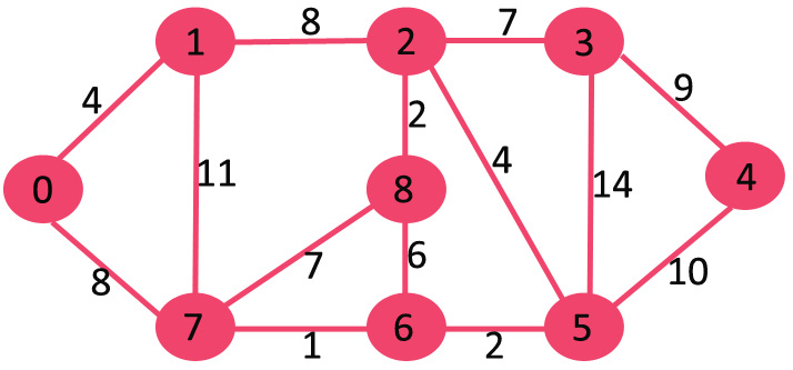
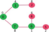
Let us understand with the following example:
The set mstSet is initially empty and
keys assigned to vertices are {0, INF, INF, INF, INF, INF, INF, INF} where INF
indicates infinite. Now pick the vertex with minimum key value. The vertex 0 is
picked, include it in mstSet. So mstSet becomes {0}. After
including to mstSet, update key values of adjacent vertices. Adjacent vertices of 0
are 1 and 7. The key values of 1 and 7 are updated as 4 and 8. Following
subgraph shows vertices and their key values, only the vertices with finite key
values are shown. The vertices included in MST are shown in green color.
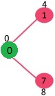
Pick the vertex with
minimum key value and not already included in MST (not in mstSET). The vertex 1
is picked and added to mstSet. So mstSet now becomes {0, 1}. Update the key
values of adjacent vertices of 1. The key value of vertex 2 becomes 8.
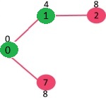
Pick the vertex with minimum key value and not already included in
MST (not in mst SET). We can either pick vertex 7 or vertex 2, let vertex 7 is
picked. So mstSet now becomes {0, 1, 7}. Update the key values of adjacent
vertices of 7. The key value of vertex 6 and 8 becomes finite (7 and 1
respectively).
Pick the vertex with
minimum key value and not already included in MST (not in mstSET). Vertex 6 is
picked. So mstSet now becomes {0, 1, 7, 6}. Update the key values of adjacent
vertices of 6. The key value of vertex 5 and 8 are updated.
We repeat the above steps until mstSet includes all vertices of
given graph. Finally, we get the following graph.
Prim’s algorithm initializes with a
node
|
Kruskal’s algorithm initiates with
an edge
|
Prim’s algorithms span from one
node to another
|
Kruskal’s algorithm select the
edges in a way that the position of the edge is not based on the last step
|
In prim’s algorithm, graph must be
a connected graph
|
Kruskal’s can function on
disconnected graphs too.
|
Prim’s algorithm has a time
complexity of O(V2)
|
Kruskal’s time complexity is
O(logV).
|
Ans 7 (i)
(A) All palindromes
·
Can you generate the string abbaabba from the languege?
(B) All odd length palindromes.
(C) Strings that begin and end with
the same symbol
·
Can you generate the string ababaaababaa from the languege?
(D) All even length palindromes.
·
Same hint as in (A)
Ans 7(ii)
Set of strings of a’s
and b’s ending with the string abb.
So L = {abb, aabb, babb,
aaabb, ababb, …………..}
Ans 7 (iii)
According to Noam Chomosky, there are four types of grammars −
Type 0, Type 1, Type 2, and Type 3. The following table shows how they differ
from each other −
Grammar Type
|
Grammar Accepted
|
Language Accepted
|
Automaton
|
Type 0
|
Unrestricted grammar
|
Recursively enumerable language
|
Turing Machine
|
Type 1
|
Context-sensitive grammar
|
Context-sensitive language
|
Linear-bounded automaton
|
Type 2
|
Context-free grammar
|
Context-free language
|
Pushdown automaton
|
Type 3
|
Regular grammar
|
Regular language
|
Finite state automaton
|
Take a look at the following illustration. It shows the scope of
each type of grammar −
Type - 3 Grammar
Type-3 grammars generate regular languages. Type-3 grammars must have a
single non-terminal on the left-hand side and a right-hand side consisting of a
single terminal or single terminal followed by a single non-terminal.
The productions must be in the form X → a or X → aY
where X, Y ∈ N (Non terminal)
and a ∈ T (Terminal)
The rule S → ε is allowed if S does
not appear on the right side of any rule.
Example
Type - 2 Grammar
Type-2 grammars generate context-free languages.
The productions must be in the form A → γ
where A ∈ N (Non terminal)
and γ ∈ (T ∪ N)* (String of terminals and non-terminals).
These languages generated by these grammars are be recognized by a
non-deterministic pushdown automaton.
Example
S → X a
X → a
X → aX
X → abc
X → ε
Type - 1 Grammar
Type-1 grammars generate context-sensitive languages. The productions must
be in the form
α A β → α γ β
where A ∈ N (Non-terminal)
and α, β, γ ∈ (T ∪ N)* (Strings of terminals and non-terminals)
The strings α and β may be
empty, but γ must be non-empty.
The rule S → ε is allowed if S does not appear on
the right side of any rule. The languages generated by these grammars are
recognized by a linear bounded automaton.
Example
Type - 0 Grammar
Type-0 grammars generate recursively enumerable languages. The productions
have no restrictions. They are any phase structure grammar including all formal
grammars.
They generate the languages that are recognized by a Turing
machine.
The productions can be in the form of α → β where α is a string of terminals and
nonterminals with at least one non-terminal and α cannot be
null. β is a string of terminals and non-terminals.
Example
S → ACaB
Bc → acB
CB → DB
aD → Db
Ans 7(iv)
In formal language theory, a context-free language
is a language generated by some context-free grammar. The set of all
context-free languages is identical to the set of languages accepted by
pushdown automata.
Proof:
If L1 and L2
are context-free languages, then each of them has a context-free grammar; call
the grammars G1 and G2.
Our proof requires that the grammars have no
non-terminals in common. So we shall subscript all of G1’s non-terminals with a
1 and subscript all of G2’s non-terminals with a 2. Now, we combine the two
grammars into one grammar that will generate the union of the two languages. To
do this, we add one new non-terminal, S, and two new productions.
S -> S1 | S2
S is the
starting non-terminal for the new union grammar and can be replaced either by
the starting non-terminal for G1 or for G2, thereby generating either a string
from L1 or from L2. Since the non-terminals of the two original
languages are completely different, and once we
begin using one of the original grammars, we must complete
the derivation using only the rules from that
original grammar. Note that there is no need for the
alphabets of the two languages to be the same. Therefore, it is proved that if
L1 and L2 are context – free languages, then L1 Union L2 is also a context –
free language.
Ans 7 (v)
Ans 8 (i) Halting Problem
Input −
A Turing machine and an input string w.
Problem −
Does the Turing machine finish computing of the string w in a
finite number of steps? The answer must be either yes or no.
Proof −
At first, we will assume that such a Turing machine exists to solve this
problem and then we will show it is contradicting itself. We will call this
Turing machine as a Halting machine that produces a ‘yes’ or
‘no’ in a finite amount of time. If the halting machine finishes in a finite
amount of time, the output comes as ‘yes’, otherwise as ‘no’.
(ii) Rice Theorem
Theorem
L = {<M> | L (M) ∈ P} is undecidable
when p, a non-trivial property of the Turing machine, is
undecidable.
If the following two properties hold, it is proved as undecidable
−
Property 1 − If M1 and M2 recognize
the same language, then either <M1> <M2> ∈ L or <M1> <M2> ∉ L
Property 2 − For some M1 and M2 such that <M1> ∈ L and <M2> ∉ L
Proof −
Let there are two Turing machines X1 and X2.
Let us assume <X1> ∈ L such that
L(X1) = φ and <X2> ∉ L.
For an input ‘w’ in a particular instant, perform the following
steps −
·
If X accepts w, then simulate X2 on x.
·
Run Z on input <W>.
·
If Z accepts <W>, Reject it;
and if Z rejects <W>, accept it.
If X accepts w, then
L(W) = L(X2) and <W> ∉ P
If M does not accept w, then
L(W) = L(X1) = φ and <W> ∈ P
Here the contradiction arises. Hence, it is undecidable.
(iii) The Post Correspondence Problem (PCP), introduced by Emil Post
in 1946, is an undecidable decision problem. The PCP problem over an alphabet ∑
is stated as follows −
Given the following two lists, M and N of
non-empty strings over ∑ −
M = (x1, x2, x3,………, xn)
N = (y1, y2, y3,………, yn)
We can say that there is a Post Correspondence Solution, if for
some i1,i2,………… ik, where 1 ≤ ij ≤
n, the condition xi1 …….xik = yi1 …….yik satisfies.
Example 1
Find whether the lists
M = (abb, aa, aaa) and N = (bba, aaa, aa)
have a Post Correspondence Solution?
Solution
|
x1
|
x2
|
x3
|
M
|
Abb
|
aa
|
aaa
|
N
|
Bba
|
aaa
|
aa
|
Here,
x2x1x3 = ‘aaabbaaa’
and y2y1y3 =
‘aaabbaaa’
We can see that
x2x1x3 = y2y1y3
Hence, the solution is i = 2, j = 1, and k = 3.
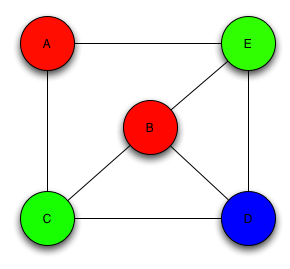
iv) K-Colourability Problem:
Vertex coloring is
the most common graph coloring problem. The problem is, given m colors, find a
way of coloring the vertices of a graph such that no two adjacent vertices are
colored using same color. The other graph coloring problems like Edge Coloring (No
vertex is incident to two edges of same color) and Face Coloring (Geographical Map Coloring) can be transformed into
vertex coloring.
Chromatic Number: The
smallest number of colors needed to color a graph G is called its chromatic
number. For example, the following can be colored minimum 3 colors.
Ans 8 (v)Independent Line Set
Independent Set
Independent sets are represented in sets, in which
· there should not be any edges adjacent to each other. There should not be any common vertex between any two edges.
· there should not be any vertices adjacent to each other. There should not be any common edge between any two vertices.
Let ‘G’ = (V, E) be a graph. A subset L of E is called an
independent line set of ‘G’ if two edges in L are adjacent. Such a set is
called an independent line set.
Example
Let us consider the following subsets −
L1 = {a,b}
L2 = {a,b} {c,e}
L3 = {a,d} {b,c}
In this example, the subsets L2 and L3 are
clearly not the adjacent edges in the given graph. They are independent line
sets. However L1 is not an independent line set, as for making
an independent line set, there should be at least two edges.
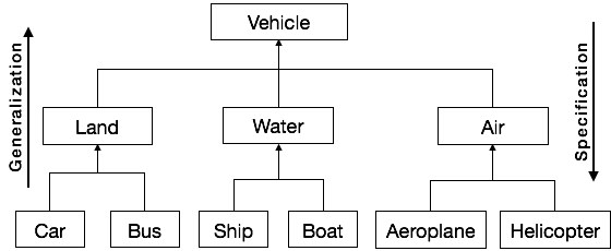


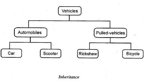
 In the same way, OOP allows one class to inherit the properties of another class or classes. The class, which is inherited by the other classes, is known as superclass or base class or parent class and the class, which inherits the properties of the base class, is called sub class or derived class or child class. The sub class can further be inherited to form other derived classes. For example, car and scooter are the derived classes of automobiles and rickshaw and bicycle are the derived classes of pulled vehicles


