MCA 2nd sem /MCS-021/Solved Assignment/Data and File Structures/2017-2018 New

Q.1.

A.1.

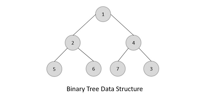
Tree represents the nodes connected by edges. We will discuss binary tree or binary search tree specifically.

Binary Tree is a special datastructure used for data storage purposes. A binary tree has a special condition that each node can have a maximum of two children. A binary tree has the benefits of both an ordered array and a linked list as search is as quick as in a sorted array and insertion or deletion operation are as fast as in linked list.

PROCEDURE CONVERT
[Given a forest of trees, it is required to convert this forest into an equivalent binary tree with a list head (HEAD)].

1. [Initialize]

HEAD <-- NODE
LPTR(HEAD) <-- NULL
RPTR(HEAD) <-- HEAD
LEVEL[1] <-- 0
LOCATION TOP <-- 1.

2. [Process the input]

Repeat thru step 6 while input is there.

3. [Input a node]

Read(LEVEL,INFO).

4. [Create a tree node]

NEW <-- NODE
LPTR(NEW) <-- RPTR(NEW) <-- NULL
DATA(NEW) <-- INFO.

5. [Compare levels]

PRED_LEVEL <-- LEVEL[TOP]
PRED_LOC <-- LOCATION[TOP]
if LEVEL > PRED_LEVEL
then LPTR(PRED_LOC) <-- NEW
else if LEVEL = PRED_LEVEL
RPTR(PRED_LOC) <-- NEW
TOP <-- TOP – 1
else
Repeat while LEVEL != PRED_LEVEL
TOP <-- TOP – 1
PRED_LEVEL <-- LEVEL[TOP]
PRED_LOC <-- LOCATION[TOP]
if PRED_LEVEL <-- LEVEL
then write (“Invalid Input”)
return



RPTR(PRED_LOC) <-- NEW
TOP <-- TOP – 1.

6. [Pushing values in stack]

TOP <-- TOP + 1
LEVEL[TOP] <-- LEVEL
LOCATION[TOP] <-- NEW.

7. [FINISH]

return. 

Q.2.

A.2. 

AVL tree is a self-balancing Binary Search Tree (BST) where the difference between heights of left and right subtrees cannot be more than one for all nodes.

An Example Tree that is an AVL Tree

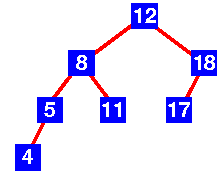
The above tree is AVL because differences between heights of left and right subtrees for every node is less than or equal to 1.

An Example Tree that is NOT an AVL Tree

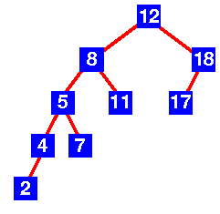
The above tree is not AVL because differences between heights of left and right subtrees for 8 and 18 is greater than 1.

Why AVL Trees?
Most of the BST operations (e.g., search, max, min, insert, delete.. etc) take O(h) time where h is the height of the BST. The cost of these operations may become O(n) for a skewed Binary tree. If we make sure that height of the tree remains O(Logn) after every insertion and deletion, then we can guarantee an upper bound of O(Logn) for all these operations. The height of an AVL tree is always O(Logn) where n is the number of nodes in the tree (See this video lecture for proof).

Insertion
To make sure that the given tree remains AVL after every insertion, we must augment the standard BST insert operation to perform some re-balancing. Following are two basic operations that can be performed to re-balance a BST without violating the BST property (keys(left) < key(root) < keys(right)). 1) Left Rotation 2) Right Rotation

T1, T2 and T3 are subtrees of the tree rooted with y (on left side) 
or x (on right side)           
                y                               x
               / \     Right Rotation          /  \
              x   T3   – – – – – – – >        T1   y 
             / \       < - - - - - - -            / \
            T1  T2     Left Rotation            T2  T3
Keys in both of the above trees follow the following order 
      keys(T1) < key(x) < keys(T2) < key(y) < keys(T3)
So BST property is not violated anywhere.

Steps to follow for insertion
Let the newly inserted node be w
1) Perform standard BST insert for w.
2) Starting from w, travel up and find the first unbalanced node. Let z be the first unbalanced node, y be the child of z that comes on the path from w to z and x be the grandchild of z that comes on the path from w to z.
3) Re-balance the tree by performing appropriate rotations on the subtree rooted with z. There can be 4 possible cases that needs to be handled as x, y and z can be arranged in 4 ways. Following are the possible 4 arrangements:
a) y is left child of z and x is left child of y (Left Left Case)
b) y is left child of z and x is right child of y (Left Right Case)
c) y is right child of z and x is right child of y (Right Right Case)
d) y is right child of z and x is left child of y (Right Left Case)

a) Left Left Case

T1, T2, T3 and T4 are subtrees.
         z                                      y 
        / \                                   /   \
       y   T4      Right Rotate (z)          x      z
      / \          - - - - - - - - ->      /  \    /  \ 
     x   T3                               T1  T2  T3  T4
    / \
  T1   T2

b) Left Right Case

     z                               z                           x
    / \                            /   \                        /  \ 
   y   T4  Left Rotate (y)        x    T4  Right Rotate(z)    y      z
  / \      - - - - - - - - ->    /  \      - - - - - - - ->  / \    / \
T1   x                          y    T3                    T1  T2 T3  T4
    / \                        / \
  T2   T3                    T1   T2

c) Right Right Case

  z                                y
 /  \                            /   \ 
T1   y     Left Rotate(z)       z      x
    /  \   - - - - - - - ->    / \    / \
   T2   x                     T1  T2 T3  T4
       / \
     T3  T4

d) Right Left Case

   z                            z                            x
  / \                          / \                          /  \ 
T1   y   Right Rotate (y)    T1   x      Left Rotate(z)   z      y
    / \  - - - - - - - - ->     /  \   - - - - - - - ->  / \    / \
   x   T4                      T2   y                  T1  T2  T3  T4
  / \                              /  \
T2   T3                           T3   T4

Implementation
Following is the implementation for AVL Tree Insertion. The following implementation uses the recursive BST insert to insert a new node. In the recursive BST insert, after insertion, we get pointers to all ancestors one by one in bottom up manner. So we don’t need parent pointer to travel up. The recursive code itself travels up and visits all the ancestors of the newly inserted node.
1) Perform the normal BST insertion.
2) The current node must be one of the ancestors of the newly inserted node. Update the height of the current node.
3) Get the balance factor (left subtree height – right subtree height) of the current node.
4) If balance factor is greater than 1, then the current node is unbalanced and we are either in Left Left case or left Right case. To check whether it is left left case or not, compare the newly inserted key with the key in left subtree root.
5) If balance factor is less than -1, then the current node is unbalanced and we are either in Right Right case or Right Left case. To check whether it is Right Right case or not, compare the newly inserted key with the key in right subtree root.

Q.3.

A.3.Sorting Techniques:-

1) Bubble Sort:-

Bubble sort is a simple sorting algorithm. This sorting algorithm is comparison-based algorithm in which each pair of adjacent elements is compared and the elements are swapped if they are not in order. This algorithm is not suitable for large data sets as its average and worst case complexity are of Ο(n²) where n is the number of items.

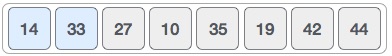
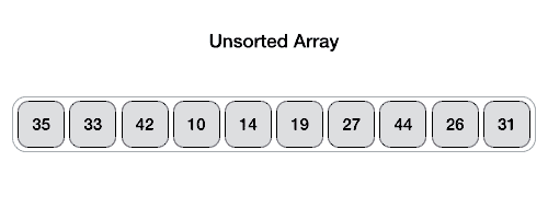
We take an unsorted array for our example. Bubble sort takes Ο(n²) time so we're keeping it short and precise.

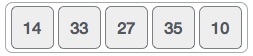
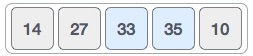
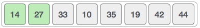
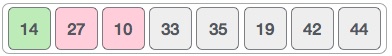
Bubble sort starts with very first two elements, comparing them to check which one is greater.

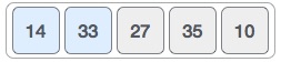
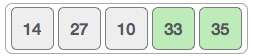
In this case, value 33 is greater than 14, so it is already in sorted locations. Next, we compare 33 with 27.

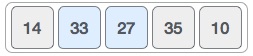
We find that 27 is smaller than 33 and these two values must be swapped.

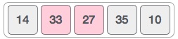
The new array should look like this −

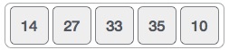
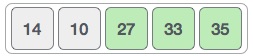
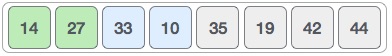
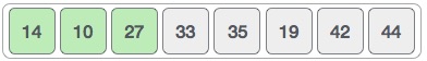
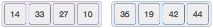
Next we compare 33 and 35. We find that both are in already sorted positions.

Then we move to the next two values, 35 and 10.

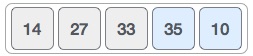
We know then that 10 is smaller 35. Hence they are not sorted.

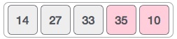
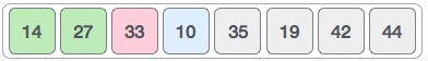
We swap these values. We find that we have reached the end of the array. After one iteration, the array should look like this −

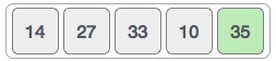
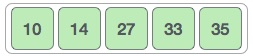
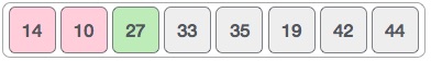
To be precise, we are now showing how an array should look like after each iteration. After the second iteration, it should look like this −

Notice that after each iteration, at least one value moves at the end.

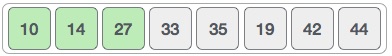
And when there's no swap required, bubble sorts learns that an array is completely sorted.

Now we should look into some practical aspects of bubble sort.

Algorithm

We assume list is an array of n elements. We further assume that swapfunction swaps the values of the given array elements.

begin BubbleSort(list)

   for all elements of list
      if list[i] > list[i+1]
         swap(list[i], list[i+1])
      end if
   end for
   
   return list
   
end BubbleSort

2) Insertion Sort:-

This is an in-place comparison-based sorting algorithm. Here, a sub-list is maintained which is always sorted. For example, the lower part of an array is maintained to be sorted.

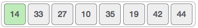
We take an unsorted array for our example.

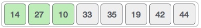
Insertion sort compares the first two elements.

It finds that both 14 and 33 are already in ascending order. For now, 14 is in sorted sub-list.

Insertion sort moves ahead and compares 33 with 27.

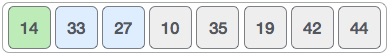
And finds that 33 is not in the correct position.

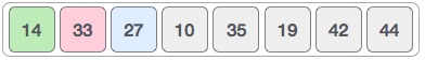
It swaps 33 with 27. It also checks with all the elements of sorted sub-list. Here we see that the sorted sub-list has only one element 14, and 27 is greater than 14. Hence, the sorted sub-list remains sorted after swapping.

By now we have 14 and 27 in the sorted sub-list. Next, it compares 33 with 10.

These values are not in a sorted order.

So we swap them.

However, swapping makes 27 and 10 unsorted.

Hence, we swap them too.

Again we find 14 and 10 in an unsorted order.

We swap them again. By the end of third iteration, we have a sorted sub-list of 4 items.

This process goes on until all the unsorted values are covered in a sorted sub-list. Now we shall see some programming aspects of insertion sort.

Algorithm

Now we have a bigger picture of how this sorting technique works, so we can derive simple steps by which we can achieve insertion sort.

Step 1 − If it is the first element, it is already sorted. return 1;
Step 2 − Pick next element
Step 3 − Compare with all elements in the sorted sub-list
Step 4 − Shift all the elements in the sorted sub-list that is greater than the 
         value to be sorted
Step 5 − Insert the value
Step 6 − Repeat until list is sorted

3) Merge Sort :-

Merge sort is a sorting technique based on divide and conquer technique. With worst-case time complexity being Ο(n log n), it is one of the most respected algorithms.

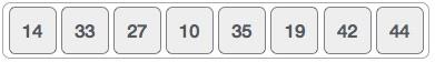
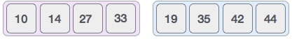
To understand merge sort, we take an unsorted array as the following −

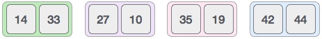
We know that merge sort first divides the whole array iteratively into equal halves unless the atomic values are achieved. We see here that an array of 8 items is divided into two arrays of size 4.

This does not change the sequence of appearance of items in the original. Now we divide these two arrays into halves.

We further divide these arrays and we achieve atomic value which can no more be divided.

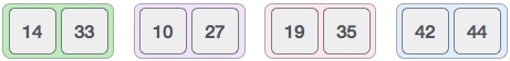
Now, we combine them in exactly the same manner as they were broken down. Please note the color codes given to these lists.

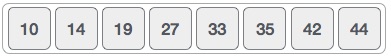
We first compare the element for each list and then combine them into another list in a sorted manner. We see that 14 and 33 are in sorted positions. We compare 27 and 10 and in the target list of 2 values we put 10 first, followed by 27. We change the order of 19 and 35 whereas 42 and 44 are placed sequentially.

In the next iteration of the combining phase, we compare lists of two data values, and merge them into a list of found data values placing all in a sorted order.

After the final merging, the list should look like this −

Now we should learn some programming aspects of merge sorting.
Algorithm
Merge sort keeps on dividing the list into equal halves until it can no more be divided. By definition, if it is only one element in the list, it is sorted. Then, merge sort combines the smaller sorted lists keeping the new list sorted too.

Step 1 − if it is only one element in the list it is already sorted, return.
Step 2 − divide the list recursively into two halves until it can no more be divided.
Step 3 − merge the smaller lists into new list in sorted order.

4) Quick Sort :-

Quick sort is a highly efficient sorting algorithm and is based on partitioning of array of data into smaller arrays. A large array is partitioned into two arrays one of which holds values smaller than the specified value, say pivot, based on which the partition is made and another array holds values greater than the pivot value.

Partition in Quick Sort

Following animated representation explains how to find the pivot value in an array.

The pivot value divides the list into two parts. And recursively, we find the pivot for each sub-lists until all lists contains only one element.

Quick Sort Pivot Algorithm
Based on our understanding of partitioning in quick sort, we will now try to write an algorithm for it, which is as follows.

Step 1 − Choose the highest index value has pivot
Step 2 − Take two variables to point left and right of the list excluding pivot
Step 3 − left points to the low index
Step 4 − right points to the high
Step 5 − while value at left is less than pivot move right
Step 6 − while value at right is greater than pivot move left
Step 7 − if both step 5 and step 6 does not match swap left and right
Step 8 − if left ≥ right, the point where they met is new pivot

Q.4.

A.4.

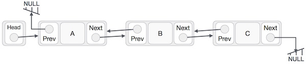
Doubly Linked List is a variation of Linked list in which navigation is possible in both ways, either forward and backward easily as compared to Single Linked List. Following are the important terms to understand the concept of doubly linked list.

Link − Each link of a linked list can store a data called an element.
Next − Each link of a linked list contains a link to the next link called Next.
Prev − Each link of a linked list contains a link to the previous link called Prev.
LinkedList − A Linked List contains the connection link to the first link called First and to the last link called Last.

Doubly Linked List Representation

As per the above illustration, following are the important points to be considered.
Doubly Linked List contains a link element called first and last.
Each link carries a data field(s) and two link fields called next and prev.
Each link is linked with its next link using its next link.
Each link is linked with its previous link using its previous link.
The last link carries a link as null to mark the end of the list.

Basic Operations
Following are the basic operations supported by a list.

Insertion − Adds an element at the beginning of the list.
Deletion − Deletes an element at the beginning of the list.
Insert Last − Adds an element at the end of the list.
Delete Last − Deletes an element from the end of the list.
Insert After − Adds an element after an item of the list.
Delete − Deletes an element from the list using the key.
Display forward − Displays the complete list in a forward manner.
Display backward − Displays the complete list in a backward manner.
Insertion Operation

Following code demonstrates the insertion operation at the beginning of a doubly linked list.
Example

//insert link at the first location
void insertFirst(int key, int data) {

   //create a link
   struct node *link = (struct node*) malloc(sizeof(struct node));
   link->key = key;
   link->data = data;
 
   if(isEmpty()) {
      //make it the last link
      last = link;
   } else {
      //update first prev link
      head->prev = link;
   }

   //point it to old first link
   link->next = head;
 
   //point first to new first link
   head = link;
}

Deletion Operation

Following code demonstrates the deletion operation at the beginning of a doubly linked list.

Example

//delete first item
struct node* deleteFirst() {

   //save reference to first link
   struct node *tempLink = head;
 
   //if only one link
   if(head->next == NULL) {
      last = NULL;
   } else {
      head->next->prev = NULL;
   }
 
   head = head->next;
 
   //return the deleted link
   return tempLink;
}

Insertion at the End of an Operation

Following code demonstrates the insertion operation at the last position of a doubly linked list.

Example

//insert link at the last location
void insertLast(int key, int data) {

   //create a link
   struct node *link = (struct node*) malloc(sizeof(struct node));
   link->key = key;
   link->data = data;
 
   if(isEmpty()) {
      //make it the last link
      last = link;
   } else {
      //make link a new last link
      last->next = link;     
      
      //mark old last node as prev of new link
      link->prev = last;
   }

   //point last to new last node
   last = link;
}