Q.1. Write an algorithm for the Implementation of a Tree?
Ans1:-
Tree represents the nodes connected by edges.Binary Tree is a special data structure used for data storage purposes. A binary tree has a special condition that each node can have a maximum of two children. A binary tree has the benefits of both an ordered array and a linked list as search is as quick as in a sorted array and insertion or deletion operation are as fast as in linked list.

Important Terms
Following are the important terms with respect to tree.
· Path − Path refers to the sequence of nodes along the edges of a tree.
· Root − The node at the top of the tree is called root. There is only one root per tree and one path from the root node to any node.
· Parent − Any node except the root node has one edge upward to a node called parent.
· Child − The node below a given node connected by its edge downward is called its child node.
· Leaf − The node which does not have any child node is called the leaf node.
· Sub-tree − Sub-tree represents the descendants of a node.
· Visiting − Visiting refers to checking the value of a node when control is on the node.
· Traversing − Traversing means passing through nodes in a specific order.
· Levels − Level of a node represents the generation of a node. If the root node is at level 0, then its next child node is at level 1, its grandchild is at level 2, and so on.
· keys − Key represents a value of a node based on which a search operation is to be carried out for a node.
Binary Search Tree Representation
Binary Search tree exhibits a special behavior. A node's left child must have a value less than its parent's value and the node's right child must have a value greater than its parent value.
We're going to implement tree using node object and connecting them through references.

Tree Node
The code to write a tree node would be similar to what is given below. It has a data part and references to its left and right child nodes.
struct node {
int data;
struct node *leftChild;
struct node *rightChild;
};
In a tree, all nodes share common construct.
BST Basic Operations
The basic operations that can be performed on a binary search tree data structure, are the following −
· Insert − Inserts an element in a tree/create a tree.
· Search − Searches an element in a tree.
· Preorder Traversal − Traverses a tree in a pre-order manner.
· Inorder Traversal − Traverses a tree in an in-order manner.
· Postorder Traversal − Traverses a tree in a post-order manner.
We shall learn creating (inserting into) a tree structure and searching a data item in a tree in this chapter. We shall learn about tree traversing methods in the coming chapter.
Insert Operation
The very first insertion creates the tree. Afterwards, whenever an element is to be inserted, first locate its proper location. Start searching from the root node, then if the data is less than the key value, search for the empty location in the left subtree and insert the data. Otherwise, search for the empty location in the right subtree and insert the data.
Algorithm
If root is NULL
then create root node
return
If root exists then
compare the data with node.data
while until insertion position is located
If data is greater than node.data
goto right subtree
else
goto left subtree
endwhile
insert data
end If
Implementation
The implementation of insert function should look like this −
void insert(int data) {
struct node *tempNode = (struct node*) malloc(sizeof(struct node));
struct node *current;
struct node *parent;
tempNode->data = data;
tempNode->leftChild = NULL;
tempNode->rightChild = NULL;
//if tree is empty, create root node
if(root == NULL) {
root = tempNode;
} else {
current = root;
parent = NULL;
while(1) {
parent = current;
//go to left of the tree
if(data < parent->data) {
current = current->leftChild;
//insert to the left
if(current == NULL) {
parent->leftChild = tempNode;
return;
}
}
//go to right of the tree
else {
current = current->rightChild;
//insert to the right
if(current == NULL) {
parent->rightChild = tempNode;
return;
}
}
}
}
}
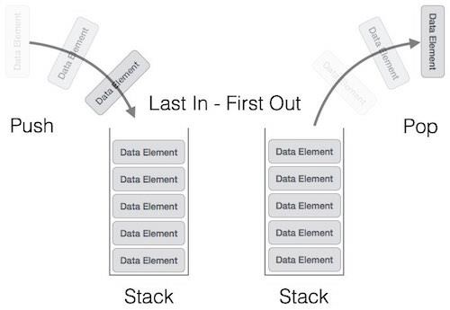
A real-world stack allows operations at one end only. For example, we can place or remove a card or plate from the top of the stack only. Likewise, Stack ADT allows all data operations at one end only. At any given time, we can only access the top element of a stack.
This feature makes it LIFO data structure. LIFO stands for Last-in-first-out. Here, the element which is placed (inserted or added) last, is accessed first. In stack terminology, insertion operation is called PUSH operation and removal operation is called POP operation.
Stack Representation
The following diagram depicts a stack and its operations −
A stack can be implemented by means of Array, Structure, Pointer, and Linked List. Stack can either be a fixed size one or it may have a sense of dynamic resizing. Here, we are going to implement stack using arrays, which makes it a fixed size stack implementation.
Basic Operations
Stack operations may involve initializing the stack, using it and then de-initializing it. Apart from these basic stuffs, a stack is used for the following two primary operations −
- push() − Pushing (storing) an element on the stack.
- pop() − Removing (accessing) an element from the stack.
When data is PUSHed onto stack.
To use a stack efficiently, we need to check the status of stack as well. For the same purpose, the following functionality is added to stacks −
- peek() − get the top data element of the stack, without removing it.
- isFull() − check if stack is full.
- isEmpty() − check if stack is empty.
Implementation multiple stacks in a Single Dimensional Array:-
#include <stdio.h>#define SIZE 10int ar[SIZE];
int top1 = -1;
int top2 = SIZE;
//Functions to push datavoid push_stack1 (int data)
{if (top1 < top2 - 1)
{ar[++top1] = data;
}else{printf ("Stack Full! Cannot Push\n");
}}void push_stack2 (int data)
{if (top1 < top2 - 1)
{ar[--top2] = data;
}else{printf ("Stack Full! Cannot Push\n");
}}//Functions to pop datavoid pop_stack1 ()
{if (top1 >= 0)
{int popped_value = ar[top1--];
printf ("%d is being popped from Stack 1\n", popped_value);
}else{printf ("Stack Empty! Cannot Pop\n");
}}void pop_stack2 ()
{if (top2 < SIZE)
{int popped_value = ar[top2++];
printf ("%d is being popped from Stack 2\n", popped_value);
}else{printf ("Stack Empty! Cannot Pop\n");
}}//Functions to Print Stack 1 and Stack 2void print_stack1 ()
{int i;
for (i = top1; i >= 0; --i)
{printf ("%d ", ar[i]);
}printf ("\n");
}void print_stack2 ()
{int i;
for (i = top2; i < SIZE; ++i)
{printf ("%d ", ar[i]);
}printf ("\n");
}int main()
{int ar[SIZE];
int i;
int num_of_ele;
printf ("We can push a total of 10 values\n");
//Number of elements pushed in stack 1 is 6//Number of elements pushed in stack 2 is 4for (i = 1; i <= 6; ++i)
{push_stack1 (i);
printf ("Value Pushed in Stack 1 is %d\n", i);
}for (i = 1; i <= 4; ++i)
{push_stack2 (i);
printf ("Value Pushed in Stack 2 is %d\n", i);
}//Print Both Stacksprint_stack1 ();
print_stack2 ();
//Pushing on Stack Fullprintf ("Pushing Value in Stack 1 is %d\n", 11);
push_stack1 (11);
//Popping All Elements From Stack 1num_of_ele = top1 + 1;
while (num_of_ele)
{pop_stack1 ();
--num_of_ele;
}//Trying to Pop From Empty Stackpop_stack1 ();
return 0;
}
Output :
gcc TwoStacksSingleArray.c
./a.out
We can push a total of 10 values
Value Pushed in Stack 1 is 1
Value Pushed in Stack 1 is 2
Value Pushed in Stack 1 is 3
Value Pushed in Stack 1 is 4
Value Pushed in Stack 1 is 5
Value Pushed in Stack 1 is 6
Value Pushed in Stack 2 is 1
Value Pushed in Stack 2 is 2
Value Pushed in Stack 2 is 3
Value Pushed in Stack 2 is 4
6 5 4 3 2 1
4 3 2 1
Pushing Value in Stack 1 is 11
Stack Full! Cannot Push
6 is being popped from Stack 1
5 is being popped from Stack 1
4 is being popped from Stack 1
3 is being popped from Stack 1
2 is being popped from Stack 1
1 is being popped from Stack 1
Stack Empty! Cannot Pop
Q.3.Write a note of not more than 5 pages summarizing the latest research in the area of "Searching Techniques".Refer to Various journals and other online resources.
Ans3. Searching Techniques :-
Searching is the process of looking for something:Finding one piece of data that has been stored withiin a whole group of data.
It is often the most time consuming part of many computer programs.
Searching is very common task in day-to-day life, where we are involved some or other time,in searching either for some needful at home or office or market, or searching a word in Dictionary.
"So, basically a search algorithm is an algorithm which accepts an argument 'a' and tries to find the corresponding data where the match of 'a' occurs in a file or in a table.
There are basically two types of Searching Techniques :-
1) Linear Search----
inear search is a very simple search algorithm. In this type of search, a sequential search is made over all items one by one. Every item is checked and if a match is found then that particular item is returned, otherwise the search continues till the end of the data collection.Algorithm
Linear Search ( Array A, Value x) Step 1: Set i to 1 Step 2: if i > n then go to step 7 Step 3: if A[i] = x then go to step 6 Step 4: Set i to i + 1 Step 5: Go to Step 2 Step 6: Print Element x Found at index i and go to step 8 Step 7: Print element not found Step 8: ExitPseudocode
procedure linear_search (list, value) for each item in the list if match item == value return the item's location end if end for end procedure2) Binary Search----Binary search is a fast search algorithm with run-time complexity of Ο(log n). This search algorithm works on the principle of divide and conquer. For this algorithm to work properly, the data collection should be in the sorted form.Binary search looks for a particular item by comparing the middle most item of the collection. If a match occurs, then the index of item is returned. If the middle item is greater than the item, then the item is searched in the sub-array to the left of the middle item. Otherwise, the item is searched for in the sub-array to the right of the middle item. This process continues on the sub-array as well until the size of the subarray reduces to zero.How Binary Search Works?
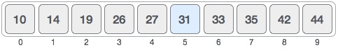
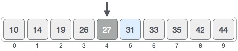
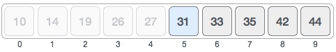
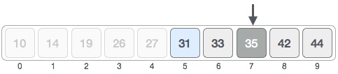
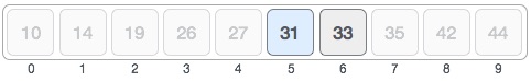
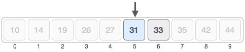
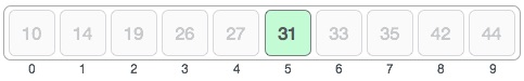
For a binary search to work, it is mandatory for the target array to be sorted. We shall learn the process of binary search with a pictorial example. The following is our sorted array and let us assume that we need to search the location of value 31 using binary search.First, we shall determine half of the array by using this formula −mid = low + (high - low) / 2Here it is, 0 + (9 - 0 ) / 2 = 4 (integer value of 4.5). So, 4 is the mid of the array.Now we compare the value stored at location 4, with the value being searched, i.e. 31. We find that the value at location 4 is 27, which is not a match. As the value is greater than 27 and we have a sorted array, so we also know that the target value must be in the upper portion of the array.We change our low to mid + 1 and find the new mid value again.low = mid + 1 mid = low + (high - low) / 2Our new mid is 7 now. We compare the value stored at location 7 with our target value 31.The value stored at location 7 is not a match, rather it is less than what we are looking for. So, the value must be in the lower part from this location.Hence, we calculate the mid again. This time it is 5.We compare the value stored at location 5 with our target value. We find that it is a match.We conclude that the target value 31 is stored at location 5.Binary search halves the searchable items and thus reduces the count of comparisons to be made to very less numbers.Pseudocode
The pseudocode of binary search algorithms should look like this −Procedure binary_search A ← sorted array n ← size of array x ← value to be searched Set lowerBound = 1 Set upperBound = n while x not found if upperBound < lowerBound EXIT: x does not exists. set midPoint = lowerBound + ( upperBound - lowerBound ) / 2 if A[midPoint] < x set lowerBound = midPoint + 1 if A[midPoint] > x set upperBound = midPoint - 1 if A[midPoint] = x EXIT: x found at location midPoint end while end procedureJournals and Online Resources (Do your Self)Q.4. What is a B- Tree ? Write a short note on its applications.Ans4. B-Tree---Introduction
Tree structures support various basic dynamic set operations including Search, Predecessor, Successor, Minimum, Maximum, Insert, and Delete in time proportional to the height of the tree. Ideally, a tree will be balanced and the height will be log n where n is the number of nodes in the tree. To ensure that the height of the tree is as small as possible and therefore provide the best running time, a balanced tree structure like a red-black tree, AVL tree, or b-tree must be used.When working with large sets of data, it is often not possible or desirable to maintain the entire structure in primary storage (RAM). Instead, a relatively small portion of the data structure is maintained in primary storage, and additional data is read from secondary storage as needed. Unfortunately, a magnetic disk, the most common form of secondary storage, is significantly slower than random access memory (RAM). In fact, the system often spends more time retrieving data than actually processing data.B-trees are balanced trees that are optimized for situations when part or all of the tree must be maintained in secondary storage such as a magnetic disk. Since disk accesses are expensive (time consuming) operations, a b-tree tries to minimize the number of disk accesses. For example, a b-tree with a height of 2 and a branching factor of 1001 can store over one billion keys but requires at most two disk accesses to search for any node (Cormen 384).
The Structure of B-Trees
Unlike a binary-tree, each node of a b-tree may have a variable number of keys and children. The keys are stored in non-decreasing order. Each key has an associated child that is the root of a subtree containing all nodes with keys less than or equal to the key but greater than the preceeding key. A node also has an additional rightmost child that is the root for a subtree containing all keys greater than any keys in the node.A b-tree has a minumum number of allowable children for each node known as the minimization factor. If t is this minimization factor, every node must have at least t - 1 keys. Under certain circumstances, the root node is allowed to violate this property by having fewer than t - 1 keys. Every node may have at most 2t - 1 keys or, equivalently, 2t children.Since each node tends to have a large branching factor (a large number of children), it is typically neccessary to traverse relatively few nodes before locating the desired key. If access to each node requires a disk access, then a b-tree will minimize the number of disk accesses required. The minimzation factor is usually chosen so that the total size of each node corresponds to a multiple of the block size of the underlying storage device. This choice simplifies and optimizes disk access. Consequently, a b-tree is an ideal data structure for situations where all data cannot reside in primary storage and accesses to secondary storage are comparatively expensive (or time consuming).Height of B-Trees
For n greater than or equal to one, the height of an n-key b-tree T of height h with a minimum degree t greater than or equal to 2,For a proof of the above inequality, refer to Cormen, Leiserson, and Rivest pages 383-384. The worst case height is O(log n). Since the "branchiness" of a b-tree can be large compared to many other balanced tree structures, the base of the logarithm tends to be large; therefore, the number of nodes visited during a search tends to be smaller than required by other tree structures. Although this does not affect the asymptotic worst case height, b-trees tend to have smaller heights than other trees with the same asymptotic height.
Operations on B-Trees
The algorithms for the search, create, and insert operations are shown below. Note that these algorithms are single pass; in other words, they do not traverse back up the tree. Since b-trees strive to minimize disk accesses and the nodes are usually stored on disk, this single-pass approach will reduce the number of node visits and thus the number of disk accesses. Simpler double-pass approaches that move back up the tree to fix violations are possible.Since all nodes are assumed to be stored in secondary storage (disk) rather than primary storage (memory), all references to a given node be be preceeded by a read operation denoted by Disk-Read. Similarly, once a node is modified and it is no longer needed, it must be written out to secondary storage with a write operation denoted by Disk-Write. The algorithms below assume that all nodes referenced in parameters have already had a corresponding Disk-Read operation. New nodes are created and assigned storage with the Allocate-Node call. The implementation details of the Disk-Read, Disk-Write, and Allocate-Node functions are operating system and implementation dependent.B-Tree-Search(x, k)
i <- 1 while i <= n[x] and k > keyi[x] do i <- i + 1 if i <= n[x] and k = keyi[x] then return (x, i) if leaf[x] then return NIL else Disk-Read(ci[x]) return B-Tree-Search(ci[x], k)The search operation on a b-tree is analogous to a search on a binary tree. Instead of choosing between a left and a right child as in a binary tree, a b-tree search must make an n-way choice. The correct child is chosen by performing a linear search of the values in the node. After finding the value greater than or equal to the desired value, the child pointer to the immediate left of that value is followed. If all values are less than the desired value, the rightmost child pointer is followed. Of course, the search can be terminated as soon as the desired node is found. Since the running time of the search operation depends upon the height of the tree, B-Tree-Search is O(logt n).B-Tree-Create(T)
B-Tree-Split-Child(x, i, y)
z <- Allocate-Node() leaf[z] <- leaf[y] n[z] <- t - 1 for j <- 1 to t - 1 do keyj[z] <- keyj+t[y] if not leaf[y] then for j <- 1 to t do cj[z] <- cj+t[y] n[y] <- t - 1 for j <- n[x] + 1 downto i + 1 do cj+1[x] <- cj[x] ci+1 <- z for j <- n[x] downto i do keyj+1[x] <- keyj[x] keyi[x] <- keyt[y] n[x] <- n[x] + 1 Disk-Write(y) Disk-Write(z) Disk-Write(x)If is node becomes "too full," it is necessary to perform a split operation. The split operation moves the median key of node x into its parent y where x is the ith child of y. A new node, z, is allocated, and all keys in x right of the median key are moved to z. The keys left of the median key remain in the original node x. The new node, z, becomes the child immediately to the right of the median key that was moved to the parent y, and the original node, x, becomes the child immediately to the left of the median key that was moved into the parent y.The split operation transforms a full node with 2t - 1 keys into two nodes with t - 1 keys each. Note that one key is moved into the parent node. The B-Tree-Split-Child algorithm will run in time O(t) where t is constant.B-Tree-Insert(T, k)
r <- root[T] if n[r] = 2t - 1 then s <- Allocate-Node() root[T] <- s leaf[s] <- FALSE n[s] <- 0 c1 <- r B-Tree-Split-Child(s, 1, r) B-Tree-Insert-Nonfull(s, k) else B-Tree-Insert-Nonfull(r, k)B-Tree-Insert-Nonfull(x, k)
i <- n[x] if leaf[x] then while i >= 1 and k < keyi[x] do keyi+1[x] <- keyi[x] i <- i - 1 keyi+1[x] <- k n[x] <- n[x] + 1 Disk-Write(x) else while i >= and k < keyi[x] do i <- i - 1 i <- i + 1 Disk-Read(ci[x]) if n[ci[x]] = 2t - 1 then B-Tree-Split-Child(x, i, ci[x]) if k > keyi[x] then i <- i + 1 B-Tree-Insert-Nonfull(ci[x], k)B-Tree-Delete
Deletion of a key from a b-tree is possible; however, special care must be taken to ensure that the properties of a b-tree are maintained. Several cases must be considered. If the deletion reduces the number of keys in a node below the minimum degree of the tree, this violation must be corrected by combining several nodes and possibly reducing the height of the tree. If the key has children, the children must be rearranged.Examples
Sample B-Tree

Searching a B-Tree for Key 21
Inserting Key 33 into a B-Tree (w/ Split) Applications Databases A database is a collection of data organized in a fashion that facilitates updating, retrieving, and managing the data. The data can consist of anything, including, but not limited to names, addresses, pictures, and numbers. Databases are commonplace and are used everyday. For example, an airline reservation system might maintain a database of available flights, customers, and tickets issued. A teacher might maintain a database of student names and grades. s t is not uncommon for a database to contain millions of records requiring many gigabytes of storage. For examples, TELSTRA, an Australian telecommunications company, maintains a customer billing database with 51 billion rows (yes, billion) and 4.2 terabytes of data. In order for a database to be useful and usable, it must support the desired operations, such as retrieval and storage, quickly. Because databases cannot typically be maintained entirely in memory, b-trees are often used to index the data and to provide fast access. For example, searching an unindexed and unsorted database containing n key values will have a worst case running time of O(n); if the same data is indexed with a b-tree, the same search operation will run in O(log n). To perform a search for a single key on a set of one million keys (1,000,000), a linear search will require at most 1,000,000 comparisons. If the same data is indexed with a b-tree of minimum degree 10, 114 comparisons will be required in the worst case. Clearly, indexing large amounts of data can significantly improve search performance. Although other balanced tree structures can be used, a b-tree also optimizes costly disk accesses that are of concern when dealing with large data sets. Concurrent Access to B-Trees Databases typically run in multiuser environments where many users can concurrently perform operations on the database. Unfortunately, this common scenario introduces complications. For example, imagine a database storing bank account balances. Now assume that someone attempts to withdraw $40 from an account containing $60. First, the current balance is checked to ensure sufficent funds. After funds are disbursed, the balance of the account is reduced. This approach works flawlessly until concurrent transactions are considered. Suppose that another person simultaneously attempts to withdraw $30 from the same account. At the same time the account balance is checked by the first person, the account balance is also retrieved for the second person. Since neither person is requesting more funds than are currently available, both requests are satisfied for a total of $70. After the first person's transaction, $20 should remain ($60 - $40), so the new balance is recorded as $20. Next, the account balance after the second person's transaction, $30 ($60 - $30), is recorded overwriting the $20 balance. Unfortunately, $70 have been disbursed, but the account balance has only been decreased by $30. Clearly, this behavior is undesirable, and special precautions must be taken.

wow truly better then best
ReplyDeleteu r better then best
ReplyDelete