MCA 4th sem /MCS-043/Solved Assignment/Advanced Database Management Systems/2016-2017 New

Q.1.(a)

A.1.(a)

ER-Diagram is a visual representation of data that describes how data is related to each other.

---

Symbols and Notations

Q.1.(b)

A.1.(b)

Q.1.(c)

A.1.(c)

Generalization is a bottom-up approach in which two lower level entities combine to form a higher level entity. In generalization, the higher level entity can also combine with other lower level entity to make further higher level entity.

Generalization is a abstracting process of viewing sets of objects as a single general 

class by concentrating on the general characteristics of the constituent sets while suppressing or ignoring their differences.
In simple terms, Generalization is a process of extracting common characteristics from two or more classes and combining them into a generalized superclass. So, it is a bottom up approach as two or more lower lever entities are combined to form a higher level entity.
The common characteristics means here attributes or methods.

---

Specialization

Specialization is opposite to Generalization. It is a top-down approach in which one higher level entity can be broken down into two lower level entity. In specialization, some higher level entities may not have lower-level entity sets at all.

Specialization may be seen as the reverse process of Generalization. Specialization is the abstracting process of introducing new characteristics to an existing class of objects to create one or more new classes of objects.
In simple terms, a group of entities  in specialization can be categorized into sub-groups based on their characteristics. So it is a top-down approach in which one higher level entity can be broken down into two lower level entity. It defines one or more subtypes of the supertypes and forming supertype/subtype relationships.

Q.1.(d)

A.1.(d) Difference Between Weak Entity And Strong Entity

The entity set which does not have sufficient attributes to form a primary key is called as Weak entity set. An entity set that has a primary key is called as Strong entity set. Consider an entity set Payment which has three attributes: payment_number, payment_date and payment_amount. Although each payment entity is distinct but payment for different loans may share the same payment number. Thus, this entity set does not have a primary key and it is an entity set. Each weak set must be a part of one-to-many relationship set.

A member of a strong entity set is called dominant entity and member of weak entity set is called as subordinate entity. A weak entity set does not have a primary key but we need a means of distinguishing among all those entries in the entity set that depend on one particular strong entity set. The discriminator of a weak entity set is a set of attributes that allows this distinction be made. For example, payment_number acts as discriminator for payment entity set. It is also called as the Partial key of the entity set.

The primary key of a weak entity set is formed by the primary key of the strong entity set on which the weak entity set is existence dependent plus the weak entity sets discriminator. In the above example {loan_number, payment_number} acts as primary key for payment entity set.

The relationship between weak entity and strong entity set is called as Identifying Relationship. In example, loan-payment is the identifying relationship for payment entity. A weak entity set is represented by doubly outlined box .and corresponding identifying relation by a doubly outlined diamond as shown in figure. Here double lines indicate total participation of weak entity in strong entity set it means that every payment must be related via loan-payment to some account. The arrow from loan-payment to loan indicates that each payment is for a single loan. The discriminator of a weak entity set is underlined with dashed lines rather than solid line.

                          

Q.1.(e)

A.1.(e)

Relational algebra is a procedural query language, which takes instances of relations as input and yields instances of relations as output. It uses operators to perform queries. An operator can be either unary or binary. They accept relations as their input and yield relations as their output. Relational algebra is performed recursively on a relation and intermediate results are also considered relations.

The fundamental operations of relational algebra are as follows −

• Select
• Project
• Union
• Set different
• Cartesian product
• Rename

We will discuss all these operations in the following sections.

Select Operation (σ)

It selects tuples that satisfy the given predicate from a relation.

Notation − σ_p(r)

Where σ stands for selection predicate and r stands for relation. p is prepositional logic formula which may use connectors like and, or, and not. These terms may use relational operators like − =, ≠, ≥, < ,  >,  ≤.

For example −

σsubject = "database"(Books)

Output − Selects tuples from books where subject is 'database'.

σsubject = "database" and price = "450"(Books)

Output − Selects tuples from books where subject is 'database' and 'price' is 450.

σsubject = "database" and price = "450" or year > "2010"(Books)

Output − Selects tuples from books where subject is 'database' and 'price' is 450 or those books published after 2010.

Project Operation (∏)

It projects column(s) that satisfy a given predicate.

Notation − ∏_{A1, A2, An} (r)

Where A₁, A₂ , A_n are attribute names of relation r.

Duplicate rows are automatically eliminated, as relation is a set.

For example −

∏subject, author (Books)

Selects and projects columns named as subject and author from the relation Books.

Union Operation (∪)

It performs binary union between two given relations and is defined as −

r ∪ s = { t | t ∈ r or t ∈ s}

Notation − r U s

Where r and s are either database relations or relation result set (temporary relation).

For a union operation to be valid, the following conditions must hold −

• r, and s must have the same number of attributes.
• Attribute domains must be compatible.
• Duplicate tuples are automatically eliminated.

∏ author (Books) ∪ ∏ author (Articles)

Output − Projects the names of the authors who have either written a book or an article or both.

Set Difference (−)

The result of set difference operation is tuples, which are present in one relation but are not in the second relation.

Notation − r − s

Finds all the tuples that are present in r but not in s.

∏ author (Books) − ∏ author (Articles)

Output − Provides the name of authors who have written books but not articles.

Cartesian Product (Χ)

Combines information of two different relations into one.

Notation − r Χ s

Where r and s are relations and their output will be defined as −

r Χ s = { q t | q ∈ r and t ∈ s}

σauthor = 'tutorialspoint'(Books Χ Articles)

Output − Yields a relation, which shows all the books and articles written by tutorialspoint.

Rename Operation (ρ)

The results of relational algebra are also relations but without any name. The rename operation allows us to rename the output relation. 'rename' operation is denoted with small Greek letter rho ρ.

Notation − ρ _x (E)

Where the result of expression E is saved with name of x.

Additional operations are −

• Set intersection
• Assignment
• Natural join

Relational Calculus

In contrast to Relational Algebra, Relational Calculus is a non-procedural query language, that is, it tells what to do but never explains how to do it.

Relational calculus exists in two forms −

Tuple Relational Calculus (TRC)

Filtering variable ranges over tuples

Notation − {T | Condition}

Returns all tuples T that satisfies a condition.

For example −

{ T.name |  Author(T) AND T.article = 'database' }

Output − Returns tuples with 'name' from Author who has written article on 'database'.

TRC can be quantified. We can use Existential (∃) and Universal Quantifiers (∀).

For example −

{ R| ∃T   ∈ Authors(T.article='database' AND R.name=T.name)}

Output − The above query will yield the same result as the previous one.

Domain Relational Calculus (DRC)

In DRC, the filtering variable uses the domain of attributes instead of entire tuple values (as done in TRC, mentioned above).

Notation −

{ a₁, a₂, a₃, ..., a_n | P (a₁, a₂, a₃, ... ,a_n)}

Where a1, a2 are attributes and P stands for formulae built by inner attributes.

For example −

{< article, page, subject > | 
 ∈ TutorialsPoint ∧ subject = 'database'}

Output − Yields Article, Page, and Subject from the relation TutorialsPoint, where subject is database.

Just like TRC, DRC can also be written using existential and universal quantifiers. DRC also involves relational operators.

The expression power of Tuple Relation Calculus and Domain Relation Calculus is equivalent to Relational Algebra.

(i) ¶ Grade(൳SubName = "Physics" And "Chemistry" from Subject)>=70

(ii) ¶ TeacherID(൳Time = "Part Time" from Teacher)>=2

Q.2.

A.2.

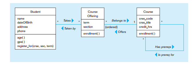
UML can be described as the successor of object oriented analysis and design.

An object contains both data and methods that control the data. The data represents the state of the object. A class describes an object and they also form hierarchy to model real world system. The hierarchy is represented as inheritance and the classes can also be associated in different manners as per the requirement.

The objects are the real world entities that exist around us and the basic concepts like abstraction, encapsulation, inheritance, polymorphism all can be represented using UML.

So UML is powerful enough to represent all the concepts exists in object oriented analysis and design. UML diagrams are representation of object oriented concepts only. So before learning UML, it becomes important to understand OO concepts in details.

Following are some fundamental concepts of object oriented world:

• Objects: Objects represent an entity and the basic building block.
• Class: Class is the blue print of an object.
• Abstraction: Abstraction represents the behavior of an real world entity.
• Encapsulation: Encapsulation is the mechanism of binding the data together and hiding them from outside world.
• Inheritance: Inheritance is the mechanism of making new classes from existing one.
• Polymorphism: It defines the mechanism to exists in different forms.

OO Analysis and Design

Object Oriented analysis can be defined as investigation and to be more specific it is the investigation of objects. Design means collaboration of identified objects.

So it is important to understand the OO analysis and design concepts. Now the most important purpose of OO analysis is to identify objects of a system to be designed. This analysis is also done for an existing system. Now an efficient analysis is only possible when we are able to start thinking in a way where objects can be identified. After identifying the objects their relationships are identified and finally the design is produced.

So the purpose of OO analysis and design can described as:

• Identifying the objects of a system.
• Identify their relationships.
• Make a design which can be converted to executables using OO languages.

There are three basic steps where the OO concepts are applied and implemented. The steps can be defined as

OO Analysis --> OO Design --> OO implementation using OO languages

Now the above three points can be described in details:

• During object oriented analysis the most important purpose is to identify objects and describing them in a proper way. If these objects are identified efficiently then the next job of design is easy. The objects should be identified with responsibilities. Responsibilities are the functions performed by the object. Each and every object has some type of responsibilities to be performed. When these responsibilities are collaborated the purpose of the system is fulfilled.
• The second phase is object oriented design. During this phase emphasis is given upon the requirements and their fulfilment. In this stage the objects are collaborated according to their intended association. After the association is complete the design is also complete.
• The third phase is object oriented implementation. In this phase the design is implemented using object oriented languages like Java, C++ etc.

Role of UML in OO design:

UML is a modeling language used to model software and non software systems. Although UML is used for non software systems the emphasis is on modeling object oriented software applications. Most of the UML diagrams discussed so far are used to model different aspects like static, dynamic etc. Now what ever be the aspect the artifacts are nothing but objects.

If we look into class diagram, object diagram, collaboration diagram, interaction diagrams all would basically be designed based on the objects.

So the relation between OO design and UML is very important to understand. The OO design is transformed into UML diagrams according to the requirement. Before understanding the UML in details the OO concepts should be learned properly. Once the OO analysis and design is done the next step is very easy. 

Q.3.

A.3. MVD:-

Classification of Dependencies in DBMS:

Partial Dependencies Second Normal Form (2NF)

TransitiveDependencies

Third Normal Form (3NF)

MultivaluedDependencies

Fourth Normal Form (4NF)

Join Dependencies Fifth Normal Form (5NF)

Inclusion Dependency

(Dependencies among the Relations/Tables

or Databases)

To understand the concept of MVD, let us consider a schema denoted as MPD (Man, Phones, Dog_Like),

Person :				Meaning of the tuples
Man(M)	Phones(P)	Dogs_Like(D)	⇒	Man M have phones P, and likes the dogs D.
M1	P1/P2	D1/D2	⇒	M1 have phones P1 and P2, and likes the dogs D1 and D2.
M2	P3	D2	⇒	M2 have phones P3, and likes the dog D2.
Key : MPD

There are no non trivial FDs because all attributes are combined forming Candidate Key i.e. MDP. The multivalued dependency is shown by “→→”. So, in  the above relation, two multivalued dependencies exists –

1. Man →→ Phones
2. Man →→ Dogs_Like

A man’s phone are independent of the dogs they like. But after converting the above relation in Single Valued Attribute, Each of a man’s phones appears with each of the dogs they like in all combinations.

Man(M)	Phones(P)	Dogs_Likes(D)
M1	P1	D1
M1	P2	D2
M2	P3	D2
M1	P1	D2
M1	P2	D1

Join Dependency:-

Let R be a relation. Let A, B, …, Z be arbitrary subsets of R’s attributes. R satisfies the JD
* ( A, B, …, Z )
if and only if R is equal to the join of its projections on A, B, …, Z.

A join dependency JD(R1, R2, …, Rn) specified on relation schema R, is a trivial JD, if one of the relation schemas Ri in JD(R1, R2, ….,Rn) is equal to R.

Join dependency is used in the following case :

When there is no lossless join decomposition of R into two relation schemas, but there is a lossless join decompositions of R into more than two relation schemas.

Point : A join dependency is very difficult in a database, hence normally not used.

Negative Example :

Consider a relation ACP(Agent, Company, Product)

ACP :				Meaning of the tuples
Agent(A)	Company(C)	Product(P)	⇒	Agent sells Company’s Products.
A1	PQR	Nut	⇒	A1 sells PQR’s Nuts and Screw.
A1	PQR	Screw
A1	XYZ	Bolt	⇒	A1 sells XYZ’s Bolts.
A2	PQR	Bolt	⇒	A2 sells PQR’s Bolts.

The table is in 4 NF as it does not contain multivalued dependency. But the relation contains redundancy as A1 is an agent for PQR twice. But there is no way of eliminating this redundancy without losing information.
Suppose that the table is decomposed into its two relations, R1 and R2.

Q.4.

A.4.

 Hash-Join: This is applicable to both the equi-joins and natural joins. A hash function h is used to

partition tuples of both relations, where h maps joining attribute (enroll no in our xample) values to

{0, 1, ..., n-1}.

The join attribute is hashed to the join-hash partitions. In the example of Figure 4 we have used

mod 100 function to hashing, and n = 100.

Once the partition tables of STUDENT and MARKS are made on the enrolment number,

then only the corresponding partitions will participate in the join as:

A STUDENT tuple and a MARKS tuple that satisfy the join condition will have the same value for

the join attributes. Therefore, they will be hashed to equivalent

partition and thus can be joined easily.

Cost calculation for Simple Hash-Join

(i) Cost of partitioning r and s: all the blocks of r and s are read once and after partitioning written

back, so cost 1 = 2 (blocks of r + blocks of s).

(ii) Cost of performing the hash-join using build and probe will require at least one block transfer

for reading the partitions

Cost 2 = (blocks of r + blocks of s)

(iii) There are a few more blocks in the main memory that may be used for evaluation, they may

be read or written back. We ignore this cost as it will be too less in comparison to cost 1 and cost

2.

Thus, the total cost = cost 1 + cost 2 = 3 (blocks of r + blocks of s)

Q.5.

A.5.

There are two intersection entities in this schema: Student/Course and Employee/Course. These handle the two many-to-many relationships: 1) between Student and Course, and 2) between Employee and Course. In the first case, a Student may take many Courses and a Course may be taken by many Students. Similarly, in the second case, an Employee (one of the types of Teachers) may teach many Courses and a Course may be taught by many Teachers. Also see more on many-to-many relationships.

1.Get Emp# of employees working on Project numbered MCS-043.

Select Emp# from Asssigned-to where Proj#=’MCS-043’;

And the output will be Emp1, Emp2

2.Get details of employees working on database projects.

 Select A.Emp#, Emp_name from A.Assigned-to, Employee where project#=’MCS-043’;

And the output will be MCA-043 Database Vinay

3.Finally create an optimal query tree for each query.

Data 1 1 2 1 3 1 4 2 5 2 6 5

Path 2 1 3 1 4 2 4 1 5 2 5 1 6 5 6 2 6 1

Q.6.

A.6.

In XML document is a basic unit of XML information composed of elements and other markup in an orderly package. An XML document can contains wide variety of data. For example, database of numbers, numbers representing molecular structure or a mathematical equation.

XML Document example

A simple document is given in the following example:

<?xml version="1.0"?> <contact-info> <name>Tanmay Patil</name> <company>TutorialsPoint</company> <phone>(011) 123-4567</phone> </contact-info>

The following image depicts the parts of XML document.

In semi-structured data, the schema or format information is mixed with the data values,since each data object can have different attributes that are not known earlier. Thus, this type ofdata is sometimes referred to as selfdescribing data.

The basic object in XML is the XML document. There are two main structuring concepts that

construct an XML document:

Elements and attributes: Attributes in XML describe elements. Elements are identified in a

document by their start tag and end tag. The tag names are enclosed between angular brackets<…>, and end tags are further identified by a backslash </…>. Complex elements are constructedfrom other elements hierarchically, whereas simple elements contain data values. Thus, there is acorrespondence between the XML textual representation and the tree structure. In the tree representation of XML, internal nodes represent complex elements, whereas leaf nodes represent simple elements. That is why the XML model is called a tree model or a hierarchical model.

Document Type Declaration (DTD): 

DTD is one of the component of XML document. A DTD is used to define the syntax and grammar of a document, that is, it defines the meaning of the document elements. XML defines a set of key words, rules, data types, etc to define the permissible structure of XML documents. In other words, we can say that you use the DTD grammar to define the grammar of your XML documents. 

XML data:

<document> Student_Data

<student>

<NAME> Vishal </NAME>

<Address> Rohini Sector 22, Delhi </Address>

</student>

<student>

<NAME> Vinod </NAME>

<Address> Rajeev Chowk, New Delhi </Address>

</student>

</document>

Q.7.
A.7.

Data Mining is defined as extracting information from huge sets of data. In other words, we can say that data mining is the procedure of mining knowledge from data. The information or knowledge extracted so can be used for any of the following applications −

• Market Analysis
• Fraud Detection
• Customer Retention
• Production Control
• Science Exploration

Data Mining Applications

Data mining is highly useful in the following domains −

• Market Analysis and Management
• Corporate Analysis & Risk Management
• Fraud Detection

Apart from these, data mining can also be used in the areas of production control, customer retention, science exploration, sports, astrology, and Internet Web Surf-Aid.

Market Analysis and Management

Listed below are the various fields of market where data mining is used −

• Customer Profiling − Data mining helps determine what kind of people buy what kind of products.
• Identifying Customer Requirements − Data mining helps in identifying the best products for different customers. It uses prediction to find the factors that may attract new customers.
• Cross Market Analysis − Data mining performs association/correlations between product sales.
• Target Marketing − Data mining helps to find clusters of model customers who share the same characteristics such as interests, spending habits, income, etc.
• Determining Customer purchasing pattern − Data mining helps in determining customer purchasing pattern.
• Providing Summary Information − Data mining provides us various multidimensional summary reports.

Corporate Analysis and Risk Management

Data mining is used in the following fields of the Corporate Sector −

• Finance Planning and Asset Evaluation − It involves cash flow analysis and prediction, contingent claim analysis to evaluate assets.
• Resource Planning − It involves summarizing and comparing the resources and spending.
• Competition − It involves monitoring competitors and market directions.

Fraud Detection

Data mining is also used in the fields of credit card services and telecommunication to detect frauds. In fraud telephone calls, it helps to find the destination of the call, duration of the call, time of the day or week, etc. It also analyzes the patterns that deviate from expected norms.

There are two forms of data analysis that can be used for extracting models describing important classes or to predict future data trends. These two forms are as follows −

• Classification
• Prediction

Classification models predict categorical class labels; and prediction models predict continuous valued functions. For example, we can build a classification model to categorize bank loan applications as either safe or risky, or a prediction model to predict the expenditures in dollars of potential customers on computer equipment given their income and occupation.

What is classification?

Following are the examples of cases where the data analysis task is Classification −

• A bank loan officer wants to analyze the data in order to know which customer (loan applicant) are risky or which are safe.
• A marketing manager at a company needs to analyze a customer with a given profile, who will buy a new computer.

In both of the above examples, a model or classifier is constructed to predict the categorical labels. These labels are risky or safe for loan application data and yes or no for marketing data.

What is prediction?

Following are the examples of cases where the data analysis task is Prediction −

Suppose the marketing manager needs to predict how much a given customer will spend during a sale at his company. In this example we are bothered to predict a numeric value. Therefore the data analysis task is an example of numeric prediction. In this case, a model or a predictor will be constructed that predicts a continuous-valued-function or ordered value.

Note − Regression analysis is a statistical methodology that is most often used for numeric prediction.

How Does Classification Works?

With the help of the bank loan application that we have discussed above, let us understand the working of classification. The Data Classification process includes two steps −

• Building the Classifier or Model
• Using Classifier for Classification

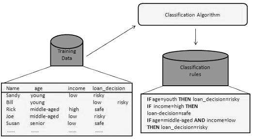
Building the Classifier or Model

• This step is the learning step or the learning phase.
• In this step the classification algorithms build the classifier.
• The classifier is built from the training set made up of database tuples and their associated class labels.
• Each tuple that constitutes the training set is referred to as a category or class. These tuples can also be referred to as sample, object or data points.

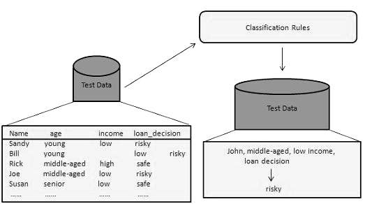
Using Classifier for Classification

In this step, the classifier is used for classification. Here the test data is used to estimate the accuracy of classification rules. The classification rules can be applied to the new data tuples if the accuracy is considered acceptable.

Classification and Prediction Issues

The major issue is preparing the data for Classification and Prediction. Preparing the data involves the following activities −

• Data Cleaning − Data cleaning involves removing the noise and treatment of missing values. The noise is removed by applying smoothing techniques and the problem of missing values is solved by replacing a missing value with most commonly occurring value for that attribute.
• Relevance Analysis − Database may also have the irrelevant attributes. Correlation analysis is used to know whether any two given attributes are related.
• Data Transformation and reduction − The data can be transformed by any of the following methods.
  • Normalization − The data is transformed using normalization. Normalization involves scaling all values for given attribute in order to make them fall within a small specified range. Normalization is used when in the learning step, the neural networks or the methods involving measurements are used.
  • Generalization − The data can also be transformed by generalizing it to the higher concept. For this purpose we can use the concept hierarchies.
  • Online transaction processing, or OLTP, is a class of information systems that facilitate and manage transaction-oriented applications, typically for data entry and retrieval transaction processing.
    The term is somewhat ambiguous; some understand a "transaction" in the context of computer or database transactions, while others (such as the Transaction Processing Performance Council) define it in terms of business or commercial transactions.^[1] OLTP has also been used to refer to processing in which the system responds immediately to user requests. An automated teller machine (ATM) for a bank is an example of a commercial transaction processing application. Online transaction processing applications are high throughput and insert or update-intensive in database management. These applications are used concurrently by hundreds of users. The key goals of OLTP applications are availability, speed, concurrency and recoverability. Reduced paper trails and the faster, more accurate forecast for revenues and expenses are both examples of how OLTP makes things simpler for businesses. However, like many modern online information technology solutions, some systems require offline maintenance, which further affects the cost–benefit analysis of on line transaction processing system.
    OLTP is typically contrasted to OLAP (online analytical processing), which is generally characterized by much more complex queries, in a smaller volume, for the purpose of business intelligence or reporting rather than to process transactions. Whereas OLTP systems process all kinds of queries (read, insert, update and delete), OLAP is generally optimized for read only and might not even support other kinds of queries.

Q.8.
A.8.

It is important that data adhere to a predefined set of rules, as determined by the database administrator or application developer. As an example of data integrity, consider the tables employees and departments and the business rules for the information in each of the tables.

Note that some columns in each table have specific rules that constrain the data contained within them.

Types of Data Integrity

This section describes the rules that can be applied to table columns to enforce different types of data integrity.

Null Rule

A null rule is a rule defined on a single column that allows or disallows inserts or updates of rows containing a null (the absence of a value) in that column.

Unique Column Values

A unique value rule defined on a column (or set of columns) allows the insert or update of a row only if it contains a unique value in that column (or set of columns).

Primary Key Values

A primary key value rule defined on a key (a column or set of columns) specifies that each row in the table can be uniquely identified by the values in the key.

Referential Integrity Rules

A referential integrity rule is a rule defined on a key (a column or set of columns) in one table that guarantees that the values in that key match the values in a key in a related table (the referenced value).

Referential integrity also includes the rules that dictate what types of data manipulation are allowed on referenced values and how these actions affect dependent values. The rules associated with referential integrity are:

• Restrict: Disallows the update or deletion of referenced data.
• Set to Null: When referenced data is updated or deleted, all associated dependent data is set to NULL.
• Set to Default: When referenced data is updated or deleted, all associated dependent data is set to a default value.
• Cascade: When referenced data is updated, all associated dependent data is correspondingly updated. When a referenced row is deleted, all associated dependent rows are deleted.
• No Action: Disallows the update or deletion of referenced data. This differs from RESTRICT in that it is checked at the end of the statement, or at the end of the transaction if the constraint is deferred. (Oracle uses No Action as its default action.)

Complex Integrity Checking

Complex integrity checking is a user-defined rule for a column (or set of columns) that allows or disallows inserts, updates, or deletes of a row based on the value it contains for the column (or set of columns).

How Oracle Enforces Data Integrity

Oracle enables you to define and enforce each type of data integrity rule defined in the previous section. Most of these rules are easily defined using integrity constraints or database triggers.

Integrity Constraints Description

An integrity constraint is a declarative method of defining a rule for a column of a table. Oracle supports the following integrity constraints:

• NOT NULL constraints for the rules associated with nulls in a column
• UNIQUE key constraints for the rule associated with unique column values
• PRIMARY KEY constraints for the rule associated with primary identification values
• FOREIGN KEY constraints for the rules associated with referential integrity. Oracle supports the use of FOREIGN KEY integrity constraints to define the referential integrity actions, including:
  • Update and delete No Action
  • Delete CASCADE
  • Delete SET NULL
• CHECK constraints for complex integrity rules

NOT NULL Integrity Constraints

By default, all columns in a table allow nulls. Null means the absence of a value. A NOT NULL constraint requires a column of a table contain no null values. For example, you can define a NOT NULL constraint to require that a value be input in the last_name column for every row of the employeestable.

Figure 21-2 illustrates a NOT NULL integrity constraint.

Figure 21-2 NOT NULL Integrity Constraints

Description of "Figure 21-2 NOT NULL Integrity Constraints"

UNIQUE Key Integrity Constraints

A UNIQUE key integrity constraint requires that every value in a column or set of columns (key) be unique—that is, no two rows of a table have duplicate values in a specified column or set of columns.

For example, in Figure 21-3 a UNIQUE key constraint is defined on the DNAME column of the dept table to disallow rows with duplicate department names.

Figure 21-3 A UNIQUE Key Constraint

Description of "Figure 21-3 A UNIQUE Key Constraint"

Unique Keys

The columns included in the definition of the UNIQUE key constraint are called the unique key. Unique key is often incorrectly used as a synonym for the terms UNIQUE key constraint or UNIQUE index. However, note that key refers only to the column or set of columns used in the definition of the integrity constraint.

If the UNIQUE key consists of more than one column, then that group of columns is said to be a composite unique key. For example, in Figure 21-4 the customer table has a UNIQUE key constraint defined on the composite unique key: the area and phone columns.

Figure 21-4 A Composite UNIQUE Key Constraint

Q.9.

A.9.

PostgreSQL (pronounced as post-gress-Q-L) is an open source relational database management system ( DBMS ) developed by a worldwide team of volunteers. PostgreSQL is not controlled by any corporation or other private entity and the source code is available free of charge.

Brief History

PostgreSQL, originally called Postgres, was created at UCB by a computer science professor named Michael Stonebraker. Stonebraker started Postgres in 1986 as a followup project to its predecessor, Ingres, now owned by Computer Associates.

1. 1977-1985: A project called INGRES was developed.
   • Proof-of-concept for relational databases
   • Established the company Ingres in 1980
   • Bought by Computer Associates in 1994
2. 1986-1994: POSTGRES
   • Development of the concepts in INGRES with a focus on object orientation and the query language Quel
   • The code base of INGRES was not used as a basis for POSTGRES
   • Commercialized as Illustra (bought by Informix, bought by IBM)
3. 1994-1995: Postgres95
   • Support for SQL was added in 1994
   • Released as Postgres95 in 1995
   • Re-released as PostgreSQL 6.0 in 1996
   • Establishment of the PostgreSQL Global Development Team

Key features of PostgreSQL

PostgreSQL runs on all major operating systems, including Linux, UNIX (AIX, BSD, HP-UX, SGI IRIX, Mac OS X, Solaris, Tru64), and Windows. It supports text, images, sounds, and video, and includes programming interfaces for C / C++ , Java , Perl , Python , Ruby, Tcl and Open Database Connectivity (ODBC).

PostgreSQL supports a large part of the SQL standard and offers many modern features including the following:

• Complex SQL queries
• SQL Sub-selects
• Foreign keys
• Trigger
• Views
• Transactions
• Multiversion concurrency control (MVCC)
• Streaming Replication (as of 9.0)
• Hot Standby (as of 9.0)

You can check official documentation of PostgreSQL to understand above-mentioned features. PostgreSQL can be extended by the user in many ways, for example by adding new:

• Data types
• Functions
• Operators
• Aggregate functions
• Index methods

Indexes are special lookup tables that the database search engine can use to speed up data retrieval. Simply put, an index is a pointer to data in a table. An index in a database is very similar to an index in the back of a book.

For example, if you want to reference all pages in a book that discuss a certain topic, you first refer to the index, which lists all topics alphabetically and are then referred to one or more specific page numbers.

An index helps speed up SELECT queries and WHERE clauses, but it slows down data input, with UPDATE and INSERT statements. Indexes can be created or dropped with no effect on the data.

Creating an index involves the CREATE INDEX statement, which allows you to name the index, to specify the table and which column or columns to index, and to indicate whether the index is in ascending or descending order.

Indexes can also be unique, similar to the UNIQUE constraint, in that the index prevents duplicate entries in the column or combination of columns on which there's an index.

The CREATE INDEX Command:

The basic syntax of CREATE INDEX is as follows:

CREATE INDEX index_name ON table_name;

Index Types

PostgreSQL provides several index types: B-tree, Hash, GiST, SP-GiST and GIN. Each index type uses a different algorithm that is best suited to different types of queries. By default, the CREATE INDEX command creates B-tree indexes, which fit the most common situations.

Single-Column Indexes:

A single-column index is one that is created based on only one table column. The basic syntax is as follows:

CREATE INDEX index_name
ON table_name (column_name);

Multicolumn Indexes:

A multicolumn index is defined on more than one column of a table. The basic syntax is as follows:

CREATE INDEX index_name
ON table_name (column1_name, column2_name);

Whether to create a single-column index or a multicolumn index, take into consideration the column(s) that you may use very frequently in a query's WHERE clause as filter conditions.

Should there be only one column used, a single-column index should be the choice. Should there be two or more columns that are frequently used in the WHERE clause as filters, the multicolumn index would be the best choice.

Unique Indexes:

Unique indexes are used not only for performance, but also for data integrity. A unique index does not allow any duplicate values to be inserted into the table. The basic syntax is as follows:

CREATE UNIQUE INDEX index_name
on table_name (column_name);

Partial Indexes:

A partial index is an index built over a subset of a table; the subset is defined by a conditional expression (called the predicate of the partial index). The index contains entries only for those table rows that satisfy the predicate. The basic syntax is as follows:

CREATE INDEX index_name
on table_name (conditional_expression);

Implicit Indexes:

Implicit indexes are indexes that are automatically created by the database server when an object is created. Indexes are automatically created for primary key constraints and unique constraints.

Example

Following is an example where we will create an index on COMPANY table for salary column:

# CREATE INDEX salary_index ON COMPANY (salary);

Now, let's list down all the indices available on COMPANY table using \d company command as follows:

# \d company

This will produce the following result, where company_pkey is an implicit index which got created when the table was created.

       Table "public.company"
 Column  |     Type      | Modifiers
---------+---------------+-----------
 id      | integer       | not null
 name    | text          | not null
 age     | integer       | not null
 address | character(50) |
 salary  | real          |
Indexes:
    "company_pkey" PRIMARY KEY, btree (id)
    "salary_index" btree (salary)

You can list down the entire indexes database wide using the \di command:

The DROP INDEX Command:

An index can be dropped using PostgreSQL DROP command. Care should be taken when dropping an index because performance may be slowed or improved.

The basic syntax is as follows:

DROP INDEX index_name;