MCA 3rd sem /MCS-031/Solved Assignment/Design and Analysis of Algorithms/2016-2017 New

Q.1.Discuss some real world problems, to which the techniques given below are applicable
(i) Divide & Conquer
(ii) Dynamic Programming
(iii) Greedy Approach

A.1.(a) Divide & Conquer:-

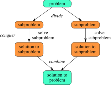
In divide and conquer approach, the problem in hand, is divided into smaller sub-problems and then each problem is solved independently. When we keep on dividing the subproblems into even smaller sub-problems, we may eventually reach a stage where no more division is possible. Those "atomic" smallest possible sub-problem (fractions) are solved. The solution of all sub-problems is finally merged in order to obtain the solution of an original problem.

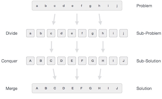
Broadly, we can understand divide-and-conquer approach in a three-step process.

Divide/Break

This step involves breaking the problem into smaller sub-problems. Sub-problems should represent a part of the original problem. This step generally takes a recursive approach to divide the problem until no sub-problem is further divisible. At this stage, sub-problems become atomic in nature but still represent some part of the actual problem.

Conquer/Solve

This step receives a lot of smaller sub-problems to be solved. Generally, at this level, the problems are considered 'solved' on their own.

Merge/Combine

When the smaller sub-problems are solved, this stage recursively combines them until they formulate a solution of the original problem. This algorithmic approach works recursively and conquer & merge steps works so close that they appear as one.

Examples

The following computer algorithms are based on divide-and-conquer programming approach −

• Merge Sort
• Quick Sort
• Binary Search
• Strassen's Matrix Multiplication
• Closest pair (points)

A.1.(b) Dynamic Programming

Dynamic programming approach is similar to divide and conquer in breaking down the problem into smaller and yet smaller possible sub-problems. But unlike, divide and conquer, these sub-problems are not solved independently. Rather, results of these smaller sub-problems are remembered and used for similar or overlapping sub-problems.

Dynamic programming is used where we have problems, which can be divided into similar sub-problems, so that their results can be re-used. Mostly, these algorithms are used for optimization. Before solving the in-hand sub-problem, dynamic algorithm will try to examine the results of the previously solved sub-problems. The solutions of sub-problems are combined in order to achieve the best solution.

So we can say that −

• The problem should be able to be divided into smaller overlapping sub-problem.
• An optimum solution can be achieved by using an optimum solution of smaller sub-problems.
• Dynamic algorithms use memorization.

The key to cutting down on the amount of work we do is to remember some of the past results so we can avoid recomputing results we already know. A simple solution is to store the results for the minimum number of coins in a table when we find them.

A.1(c) Greedy Algorithms

An algorithm is designed to achieve optimum solution for a given problem. In greedy algorithm approach, decisions are made from the given solution domain. As being greedy, the closest solution that seems to provide an optimum solution is chosen.

Greedy algorithms try to find a localized optimum solution, which may eventually lead to globally optimized solutions. However, generally greedy algorithms do not provide globally optimized solutions.

Counting Coins

This problem is to count to a desired value by choosing the least possible coins and the greedy approach forces the algorithm to pick the largest possible coin. If we are provided coins of ₹ 1, 2, 5 and 10 and we are asked to count ₹ 18 then the greedy procedure will be −

• 1 − Select one ₹ 10 coin, the remaining count is 8
• 2 − Then select one ₹ 5 coin, the remaining count is 3
• 3 − Then select one ₹ 2 coin, the remaining count is 1
• 3 − And finally, the selection of one ₹ 1 coins solves the problem

Though, it seems to be working fine, for this count we need to pick only 4 coins. But if we slightly change the problem then the same approach may not be able to produce the same optimum result.

For the currency system, where we have coins of 1, 7, 10 value, counting coins for value 18 will be absolutely optimum but for count like 15, it may use more coins than necessary. For example, the greedy approach will use 10 + 1 + 1 + 1 + 1 + 1, total 6 coins. Whereas the same problem could be solved by using only 3 coins (7 + 7 + 1)

Hence, we may conclude that the greedy approach picks an immediate optimized solution and may fail where global optimization is a major concern.

Examples

Most networking algorithms use the greedy approach. Here is a list of few of them −

• Travelling Salesman Problem
• Prim's Minimal Spanning Tree Algorithm
• Kruskal's Minimal Spanning Tree Algorithm
• Dijkstra's Minimal Spanning Tree Algorithm
• Graph - Map Coloring
• Graph - Vertex Cover
• Knapsack Problem
• Job Scheduling Problem

Q.2.Two algorithms A1 and A2 run on the same machine. The running time of A1 is 100 n and running time of A2 is 2n. For what value of n2, A1 runs faster than A2 ? If running time of A1 is changed to 100 n30, then what could be the possible value of n. You can use any spreadsheet software to plot the graph nVS A1 &A2 running time, to analyse the results.

A.2. Algorithm A1 :  Run time:  100 * n

Algorithm A2 : Run time :  2ⁿ

Let n = 2ˣ      =>   Log₂ n = x 

we want  the data size n such that  100 * n < 2ⁿ

=>  Log₂ (100 2ˣ) < Log₂ 2ⁿ   = n
=>  Log₂ 100 + x  < 2ˣ
=>   2ˣ - x > 6.69
let us try x = 2, 3, 4.. .It is easy to see that x is between 3 and 4.
So n is between 8 and 16.

  100 * n < 2ⁿ 
for n = 9,  we have  900 > 512
 we get  n = 10,  as   1000 < 1024..

So  for n = 10, A1 runs faster than A2.
-----------

If A1 is changed to  100 n + 30,  then
A1 will be faster than A2  for  n = 11  as
       100 *10 +30 > 2¹⁰ 
        100 * 11 + 30 < 2¹¹

Q.3.Use Principle of Mathematical induction to show that the polynomial P(X) = X3 – X, is divisible by 6, where X is a non-negative integer.

A.3. Principle of Mathematical Induction:-

Mathematical induction, is a technique for proving results or establishing statements for natural numbers. This part illustrates the method through a variety of examples.

Definition

Mathematical Induction is a mathematical technique which is used to prove a statement, a formula or a theorem is true for every natural number.

The technique involves two steps to prove a statement, as stated below −

Step 1(Base step) − It proves that a statement is true for the initial value.

Step 2(Inductive step) − It proves that if the statement is true for the n^thiteration (or number n), then it is also true for (n+1)^th iteration ( or number n+1).

How to Do It

Step 1 − Consider an initial value for which the statement is true. It is to be shown that the statement is true for n = initial value.

Step 2 − Assume the statement is true for any value of n = k. Then prove the statement is true for n = k+1. We actually break n = k+1 into two parts, one part is n = k (which is already proved) and try to prove the other part.

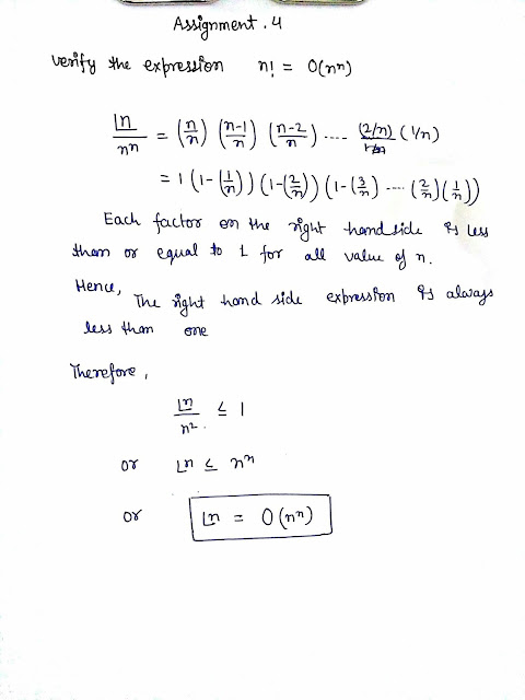
Q.4.Verify the expression n! = 0(n^n).

A.4.In mathematics, the factorial of a non-negative integer n, denoted by n!, is the product of all positive integers less than or equal to n. For example,

${\displaystyle 5!=5\times 4\times 3\times 2\times 1=120.\ }$

The value of 0! is 1, according to the convention for an empty product.^[1]

The factorial operation is encountered in many areas of mathematics, notably in combinatorics, algebra, and mathematical analysis. Its most basic occurrence is the fact that there are n! ways to arrange n distinct objects into a sequence (i.e., permutations of the set of objects). This fact was known at least as early as the 12th century, to Indian scholars.Fabian Stedman, in 1677, described factorials as applied to change ringing. After describing a recursive approach, Stedman gives a statement of a factorial (using the language of the original):

Now the nature of these methods is such, that the changes on one number comprehends [includes] the changes on all lesser numbers, ... insomuch that a compleat Peal of changes on one number seemeth to be formed by uniting of the compleat Peals on all lesser numbers into one entire body;

The notation n! was introduced by Christian Kramp in 1808.^[5]

Q.5.Determine the complexity of following sorting algorithms(i) Quick sort(ii) Merge sort(iii) Bubble sort(iv) Heap sort

A.5. Algorithmic complexity is concerned about how fast or slow particular algorithm performs. We define complexity as a numerical function T(n) - time versus the input size n. We want to define time taken by an algorithm without depending on the implementation details. But you agree that T(n) does depend on the implementation! A given algorithm will take different amounts of time on the same inputs depending on such factors as: processor speed; instruction set, disk speed, brand of compiler and etc. The way around is to estimate efficiency of each algorithm asymptotically. We will measure time T(n) as the number of elementary "steps" (defined in any way), provided each such step takes constant time.

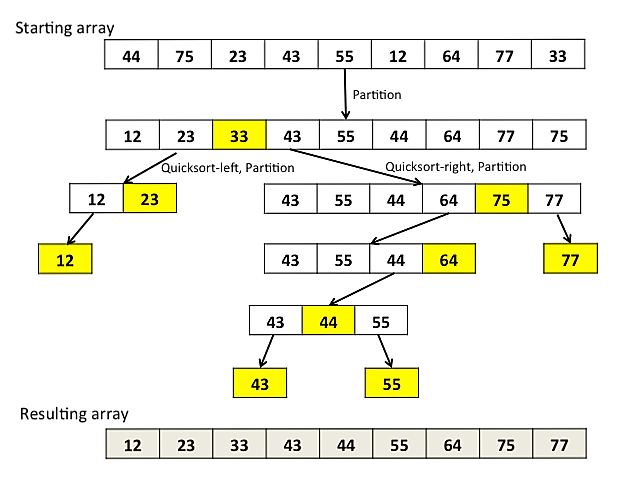
(i) Quick sort is a highly efficient sorting algorithm and is based on partitioning of array of data into smaller arrays. A large array is partitioned into two arrays one of which holds values smaller than the specified value, say pivot, based on which the partition is made and another array holds values greater than the pivot value.

Quick sort partitions an array and then calls itself recursively twice to sort the two resulting subarrays. This algorithm is quite efficient for large-sized data sets as its average and worst case complexity are of Ο(n²), where n is the number of items.

(ii) Merge Sort  is a sorting technique based on divide and conquer technique. With worst-case time complexity being Ο(n log n), it is one of the most respected algorithms.

Merge sort first divides the array into equal halves and then combines them in a sorted manner.

How Merge Sort Works?

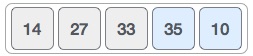
To understand merge sort, we take an unsorted array as the following −

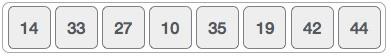
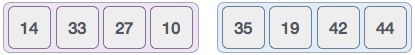
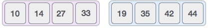
We know that merge sort first divides the whole array iteratively into equal halves unless the atomic values are achieved. We see here that an array of 8 items is divided into two arrays of size 4.

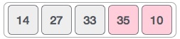
This does not change the sequence of appearance of items in the original. Now we divide these two arrays into halves.

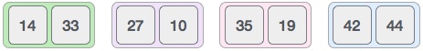
We further divide these arrays and we achieve atomic value which can no more be divided.

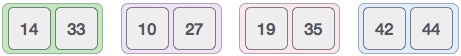
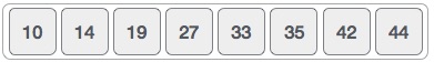
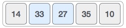
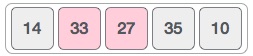
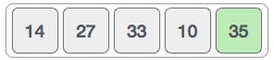
Now, we combine them in exactly the same manner as they were broken down. Please note the color codes given to these lists.

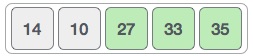
We first compare the element for each list and then combine them into another list in a sorted manner. We see that 14 and 33 are in sorted positions. We compare 27 and 10 and in the target list of 2 values we put 10 first, followed by 27. We change the order of 19 and 35 whereas 42 and 44 are placed sequentially.

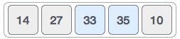
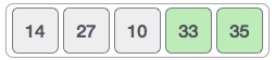
In the next iteration of the combining phase, we compare lists of two data values, and merge them into a list of found data values placing all in a sorted order.

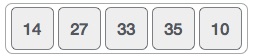
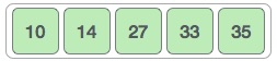
After the final merging, the list should look like this −

(iii) Bubble Sort is a simple sorting algorithm. This sorting algorithm is comparison-based algorithm in which each pair of adjacent elements is compared and the elements are swapped if they are not in order. This algorithm is not suitable for large data sets as its average and worst case complexity are of Ο(n²) where n is the number of items.

How Bubble Sort Works?

We take an unsorted array for our example. Bubble sort takes Ο(n²) time so we're keeping it short and precise.

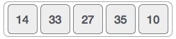
Bubble sort starts with very first two elements, comparing them to check which one is greater.

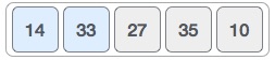
In this case, value 33 is greater than 14, so it is already in sorted locations. Next, we compare 33 with 27.

We find that 27 is smaller than 33 and these two values must be swapped.

The new array should look like this −

Next we compare 33 and 35. We find that both are in already sorted positions.

Then we move to the next two values, 35 and 10.

We know then that 10 is smaller 35. Hence they are not sorted.

We swap these values. We find that we have reached the end of the array. After one iteration, the array should look like this −

To be precise, we are now showing how an array should look like after each iteration. After the second iteration, it should look like this −

Notice that after each iteration, at least one value moves at the end.

And when there's no swap required, bubble sorts learns that an array is completely sorted.

(iv) Heap Sort is one of the best sorting methods being in-place and with no quadratic worst-case scenarios. Heap sort algorithm is divided into two basic parts :

• Creating a Heap of the unsorted list.
• Then a sorted array is created by repeatedly removing the largest/smallest element from the heap, and inserting it into the array. The heap is reconstructed after each removal.

Here is the array: 15, 19, 10, 7, 17, 6

1. Building the heap tree
The array represented as a tree, complete but not ordered:


Start with the rightmost node at height 1 - the node at position 3 = Size/2.
It has one greater child and has to be percolated down:
After processing array[3] the situation is:
Next comes array[2]. Its children are smaller, so no percolation is needed.


The last node to be processed is array[1]. Its left child is the greater of the children.
The item at array[1] has to be percolated down to the left, swapped with array[2].
As a result the situation is:
The children of array[2] are greater, and item 15 has to be moved down further, swapped with array[5].
Now the tree is ordered, and the binary heap is built.

2. Sorting - performing deleteMax operations:
1. Delete the top element 19.

1.1. Store 19 in a temporary place. A hole is created at the top


1.2. Swap 19 with the last element of the heap.
As 10 will be adjusted in the heap, its cell will no longer be a part of the heap.
Instead it becomes a cell from the sorted array

1.3. Percolate down the hole
1.4. Percolate once more (10 is less that 15, so it cannot be inserted in the previous hole)



Now 10 can be inserted in the hole


2. DeleteMax the top element 17

2.1. Store 17 in a temporary place. A hole is created at the top


2.2. Swap 17 with the last element of the heap. As 10 will be adjusted in the heap, its cell will no longer be a part of the heap.

Instead it becomes a cell from the sorted array
2.3. The element 10 is less than the children of the hole, and we percolate the hole down:



2.4. Insert 10 in the hole

3. DeleteMax 16

3.1. Store 16 in a temporary place. A hole is created at the top



3.2. Swap 16 with the last element of the heap. 

As 7 will be adjusted in the heap, its cell will no longer be a part of the heap.
Instead it becomes a cell from the sorted array
3.3. Percolate the hole down (7 cannot be inserted there - it is less than the children of the hole)
3.4. Insert 7 in the hole
4. DeleteMax the top element 15

4.1. Store 15 in a temporary location. A hole is created.



4.2. Swap 15 with the last element of the heap. 

As 10 will be adjusted in the heap, its cell will no longer be a part of the heap.
Instead it becomes a position from the sorted array
4.3. Store 10 in the hole (10 is greater than the children of the hole)
5. DeleteMax the top element 10.

5.1. Remove 10 from the heap and store it into a temporary location.



5.2. Swap 10 with the last element of the heap. 

As 7 will be adjusted in the heap, its cell will no longer be a part of the heap. Instead it becomes a cell from the sorted array



5.3. Store 7 in the hole (as the only remaining element in the heap



7 is the last element from the heap, so now the array is sorted

Q.6.Find the product of two numbers X1 = 732912 and X2 = 1026732 by using Karatsuba’s Method

A.6. 
The Karatsuba algorithm is a fast multiplication algorithm. It was discovered by Anatoly Karatsuba in 1960 and published in 1962.It reduces the multiplication of two n-digit numbers to at most ${\displaystyle n^{\log _{2}3}\approx n^{1.585}}$ single-digit multiplications in general (and exactly ${\displaystyle n^{\log _{2}3}}$ when n is a power of 2). It is therefore faster than the classical algorithm, which requires n² single-digit products. For example, the Karatsuba algorithm requires 3¹⁰ = 59,049 single-digit multiplications to multiply two 1024-digit numbers (n = 1024 = 2¹⁰), whereas the classical algorithm requires (2¹⁰)² = 1,048,576.







Q.7.Write Strassen’s Algorithm ? What are the limitation of Strassen’s Algorithim. Apply Strassen’s Algorithm to multiply two matrices A1 & A2 given below 

A = [5  6]      B = [-7  6]
       [-4  3]          [5  9]


A.7. Strassen's Algorithm :-




/* MULTIPLIES A and B =============
 using Strassen's O(n^2.81) method
   A = [5  6]      B = [-7  6]
       [-4  3]          [5  9]
     
 C = A * B = ?
 =================================*/


// Step 1: Split A and B into half-sized matrices of size 1x1 (scalars).
def a11 = 5
def a12 = 6
def a21 = -4
def a22 = 3
def b11 = -7
def b12 = 6
def b21 = 5
def b22 = 9


// Define the "S" matrix.
def s1 = b12 - b22 // -3
def s2 = a11 + a12 // 11
def s3 = a21 + a22 // -1
def s4 = b21 - b11 // 12
def s5 = a11 + a22 // 8
def s6 = b11 + b22 // 2
def s7 = a12 - a22 // -2
def s8 = b21 + b22 // 3
def s9 = a11 - a21 // 0
def s10 = b11 + b12 // -1


// Define the "P" matrix.
def p1 = a11 * s1 // -15
def p2 = s2 * b22 // 99
def p3 = s3 * b11 // 7
def p4 = a22 * s4 // 36
def p5 = s5 * s6 // 16
def p6 = s7 * s8 // -6
def p7 = s9 * s10 // 0


// Fill in the resultant "C" matrix.
def c11 = p5 + p4 - p2 + p6 // -41
def c12 = p1 + p2 //  84
def c21 = p3 + p4 //  43
def c22 = p5 + p1 - p3 - p7 // 8


/* RESULT: =================
     C = [ -41   84]
         [ 43     8]



Q.8.Perform following tasks
(a) Write Kleene closure of {aa, b}(b) Find regular expression for language {⋀, a, abb, abbbb, ….}

A.8.
(a) Kleene closure:-

Kleene Star

• Definition − The Kleene star, ∑*, is a unary operator on a set of symbols or strings, ∑, that gives the infinite set of all possible strings of all possible lengths over ∑ including λ.
• Representation − ∑* = ∑₀ ∪ ∑₁ ∪ ∑₂ ∪……. where ∑_p is the set of all possible strings of length p.
• Example − If ∑ = {a, b}, ∑* = {λ, a, b, aa, ab, ba, bb,………..}

Kleene Closure / Plus

• Definition − The set ∑⁺ is the infinite set of all possible strings of all possible lengths over ∑ excluding λ.
• Representation − ∑⁺ = ∑₁ ∪ ∑₂ ∪ ∑₃ ∪…….
  ∑⁺ = ∑* − { λ }
• Example − If ∑ = { a, b } , ∑⁺ = { a, b, aa, ab, ba, bb,………..}

**********   Kleene closure of {aa, b} = {a,aa,ab,aab,baa,...}



(b) Regular Expression :-
Language Concepts Review
We use language definitions as:
1) Testers: given a word, w, is w in the language?
2) Generators: generate all the words in the langauge.
Language definition formats:
1) Set notation: a) List of elements. Example: L1 = {aaa, bbb, ccc, ....}
b) Math formulas. Example: L2 = {an
bn
| n>= 0}
2) Recursive definition.
3) Regular expressions
Regular Expressions
Using only the letters of the alphabet Σ and these operators (kleene closure *
, positive closure +
, OR + and (
) for grouping), we can form expressions to describe words of a class of language called Regular
languages.
Examples:
Given Σ = {a, b, c}
Regular Expressions Words in the Langauge as described by the regular expressions
a {a}
ab {ab} <- concatenation
a + b {a, b}
a* {λ, a, aa, aaa, aaaa, .....}
a*b* {λ, a, b, ab, aab, aabb, .....}
(ab)* {λ, ab, abab, ababab.....}
((a+b) c)* {λ, ac, bc, acac, acbc, bcbc....}
Definition of Regular Expressions:
Given Σ:
1) ∅, λ, and all elements of Σ are Regular Expressions (primitive expressions)
2) if r1 and r2 are regular expressions, so are r1+r2, r1r2, r1* and (r1)
Example problems
Two types of problems:
1) Given a regular expression, describe the language defined by the regular expression.
2) Given a regular language, use the regular expression to describe the language

 Regular expression for language {⋀, a, abb, abbbb, ….}

{⋀, a, abb, abbbb, ….} = (ab)* b+




Q.9.Write short note on NP complete and NP Hard problems, give suitable example for each.

A.9.  NP complete

A polynomial algorithm is “faster” than an exponential algorithm. As n grows aⁿ (exponential) always grows faster than n^k (polynomial),
i.e. for any values of a and k, after n> certain integer n₀, it is true that aⁿ > n^k.
Even 2ⁿ grows faster than n¹⁰⁰⁰ at some large value of n. The former functions are exponential and the later functions are polynomial.


It seems that for some problems we just may not have any polynomial algorithm at all (as in the information theoretic bound)! The theory of NP-completeness is about this issue, and in general the computational complexity theory addresses it.



Solvable Problems



Some problems are even unsolvable/ undecidable algorithmically, so you cannot write a computer program for them.


Example. Halting problem: Given an algorithm as input, determine if it has an infinite loop.


There does not exist any general-purpose algorithm for this problem.
Suppose (contradiction) there is an algorithm H that can tell if any algorithm X halts or not, i.e., H(X) scans X and returns True iff X does halt.
Then, write
P(X):                              // X is any “input algorithm” to P
while (H(X)) { };             // condition is true only when X terminates
return;                            // P terminates
End.


Then, provide P itself as the input X to the algorithm [i.e., P(P) ]:  what happens?!
H cannot return T/F for input P, there cannot exist such H.
It is equivalent to the truth value of the sentence “This sentence is a lie.”


Note (1), we are considering Problems (i.e., for all instances of the problem) as opposed to some instances of the problem. For some sub-cases you may be able to solve the halting problem, but you cannot have an algorithm, which would solve the halting problem for ALL input.


Different types of problems:  decision problems, optimization problems, …
Decision problems: Output is True/False.


Decision Problem <-> corresponding optimization problem.
Example of 0-1 Knapsack Decision (KSD) problem:
Input: KS problem + a profit value p
Output: Answer the question "does there exist a knapsack with profit ³ p?"


Algorithms are also inter-operable between a problem and its corresponding decision problem.


Solve a KSD problem K, using an optimizing algorithm:
Algorithm-Optimization-KS (first part of K without given profit p)  return optimal profit o
if p³o then return TRUE  else return FALSE.


Solve a KS problem N, using a decision algorithm:
For (o = Sum-of-all-objects-profit;   o>0;   o = o - delta)  do  // do a linear search, for a small delta
  If (Algorithm-Decision-KS (N, o) ) then continue
   Else return  (the last value of o, before failure, in the above step);  
Endfor.   // a binary search would be faster!!


 The complexity theory is developed over Decision problems, but valid for other problems as well. We will often use other types of problems as examples.



NP-HARD PROBLEMS



As stated before, if one finds any poly-algorithm for any NP-hard problem, then
We would be able to write polynomial algorithm for each of NP-class problems, or
NP-class = P-class will be proved (in other words, poly-algorithms would be found for all NP-class problems).


Unfortunately, neither anyone could find any poly algorithm for any NP-hard problem (which would signify that P-class = NP-class);
nor anyone could prove an exponential information-theoretic bound for any NP-complete problem, say problem L (which would signify that L is in NP but not in P, or in other words that would prove that P-class Ì NP-class). The NP-hard problems are the best candidate for finding such counter-examples. 


As a result, when we say a problem X (say, the KSD problem) is NP-complete, all we mean is that
IF one finds a poly-alg for X, THEN all the NP-class problems would have poly algorithm.
We also mean, that it is UNLIKELY that there would be any poly-algorithm found for X.


NP is a mathematical conjecture currently (YET to be proved as a theorem, see above though).
Based on this conjecture many new results about the complexity-structure of computational problems have been obtained.
Note this very carefully: NP (as yet in history) does NOT stand for “non-polynomial.”




There exist other hierarchies. For example, all problems, which need polynomial memory-space (rather than time) form PSPACE problems. Poly-time algorithm will not need more than poly-space, but the reverse may not be necessarily true. Answer to this question is not known. There exists a chain of poly-transformations from all PSPACE problems to the elements of a subset of it. That subset is called PSPACE-complete. PSPACE-complete problems may lie outside NP-class, and may be harder than the NP-complete problems. Example: Quantified Boolean Formula (first-order logic) is PSPACE-complete.



Q.10. Discuss the following with suitable example
(i) Halting problem,(ii) Turing machine,(iii) Push down automata.

A.10 

(i) Halting Problem :-

Input − A Turing machine and an input string w.
Problem − Does the Turing machine finish computing of the string w in a finite number of steps? The answer must be either yes or no.
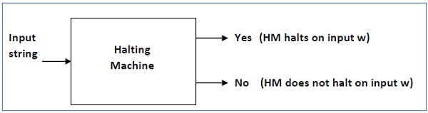
Proof − At first, we will assume that such a Turing machine exists to solve this problem and then we will show it is contradicting itself. We will call this Turing machine as a Halting machine that produces a ‘yes’ or ‘no’ in a finite amount of time. If the halting machine finishes in a finite amount of time, the output comes as ‘yes’, otherwise as ‘no’. The following is the block diagram of a Halting machine −

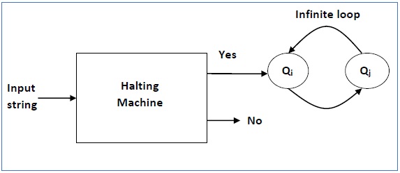
Now we will design an inverted halting machine (HM)’ as −
• If H returns YES, then loop forever.
• If H returns NO, then halt.
The following is the block diagram of an ‘Inverted halting machine’ −

Further, a machine (HM)₂ which input itself is constructed as follows −
• If (HM)₂ halts on input, loop forever.
• Else, halt.

(ii) Turing Machine :-

A Turing Machine (TM) is a mathematical model which consists of an infinite length tape divided into cells on which input is given. It consists of a head which reads the input tape. A state register stores the state of the Turing machine. After reading an input symbol, it is replaced with another symbol, its internal state is changed, and it moves from one cell to the right or left. If the TM reaches the final state, the input string is accepted, otherwise rejected.
A TM can be formally described as a 7-tuple (Q, X, ∑, δ, q₀, B, F) where −
• Q is a finite set of states
• X is the tape alphabet
• ∑ is the input alphabet
• δ is a transition function; δ : Q × X → Q × X × {Left_shift, Right_shift}.
• q₀ is the initial state
• B is the blank symbol
• F is the set of final states
Comparison with the previous automaton
The following table shows a comparison of how a Turing machine differs from Finite Automaton and Pushdown Automaton.
Machine	Stack Data Structure	Deterministic?
Finite Automaton	N.A	Yes
Pushdown Automaton	Last In First Out(LIFO)	No
Turing Machine	Infinite tape	Yes
Example of Turing machine
Turing machine M = (Q, X, ∑, δ, q₀, B, F) with
• Q = {q₀, q₁, q₂, q_f}
• X = {a, b}
• ∑ = {1}
• q₀ = {q₀}
• B = blank symbol
• F = {q_f }

(iii) Push Down Automata :-

A pushdown automaton is a way to implement a context-free grammar in a similar way we design DFA for a regular grammar. A DFA can remember a finite amount of information, but a PDA can remember an infinite amount of information.
Basically a pushdown automaton is −
"Finite state machine" + "a stack"
A pushdown automaton has three components −
• an input tape,
• a control unit, and
• a stack with infinite size.
The stack head scans the top symbol of the stack.
A stack does two operations −
• Push − a new symbol is added at the top.
• Pop − the top symbol is read and removed.
A PDA may or may not read an input symbol, but it has to read the top of the stack in every transition.

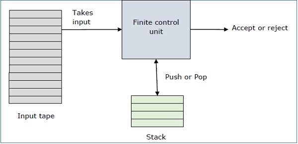
A PDA can be formally described as a 7-tuple (Q, ∑, S, δ, q₀, I, F) −
• Q is the finite number of states
• ∑ is input alphabet
• S is stack symbols
• δ is the transition function: Q × (∑ ∪ {ε}) × S × Q × S*
• q₀ is the initial state (q₀ ∈ Q)
• I is the initial stack top symbol (I ∈ S)
• F is a set of accepting states (F ∈ Q)
The following diagram shows a transition in a PDA from a state q₁ to state q₂, labeled as a,b → c −

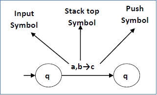
This means at state q₁, if we encounter an input string ‘a’ and top symbol of the stack is ‘b’, then we pop ‘b’, push ‘c’ on top of the stack and move to state q₂.